Analysis and visualization of BBS data using the tidyverse
Contributors: Michael T. Hallworth
Installing Required Libraries
The libraries needed for these activities are: sf tidyverse mapsInstalling the packages
If installing these packages for the first time consider addingdependencies=TRUE
install.packages("sf",dependencies = TRUE)install.packages("tidyverse",dependencies = TRUE)install.packages("maps",dependencies = TRUE)Download R script Last modified: 2019-09-20 18:26:28
This activity will introduce more advanced manipulation of spatial data using sf and the tidyverse. See introductions to spatial predicates and working with sf objects for more background information on these topics.
Breeding Bird Survey data
In this tutorial, we will use data from the North American Breeding Bird Survey to highlight some additional topics related to the creation, manipulation, and visualization of spatial objects using the sf package and the tidyverse. The raw BBS data contains three files containing, respectively, spatial information for each route, the raw counts for each species in each year on each route, and weather/observer information for each count. The raw data (with a few modifications to reduce size and unnecessary fields) are included with this tutorial.
To start, let’s load the necessary packages and read in the BBS spatial information:
library(sf)
library(tidyverse)

### Load data.frame containing the BBS spatial information
load("../Spatial_Layers/bbs_xy.rda")

### Note the columns containing lat/long for each route
head(bbs_xy)
##   countrynum statenum Route       RouteName Active Latitude Longitude
## 1        840        2     1      ST FLORIAN      1 34.86869 -87.60414
## 2        840        2     2       HILLSBORO      0 34.63867 -87.19129
## 3        840        2     3        FLORENCE      0 34.80000 -87.73333
## 4        840        2     4           TRADE      1 34.02979 -87.05924
## 5        840        2     5         SUMMITT      0 34.20167 -86.49341
## 6        840        2     6 VALHERMOSO SPGS      1 34.50129 -86.68555
##   Stratum BCR LandTypeID RouteTypeID RouteTypeDetailId  routeID
## 1      14  27          0           1                 1 84002001
## 2      14  24          0           1                 1 84002002
## 3      14  24          0           1                 1 84002003
## 4      13  28          0           1                 1 84002004
## 5      13  28          0           1                 1 84002005
## 6      14  24          0           1                 1 84002006
Next we convert bbs_xy to class sf. Remember, we need to specify which columns contain the coordinates for each route and (optionally) provide a CRS:
### Convert to `sf`
bbs_xy_sf <- st_as_sf(bbs_xy, coords = c("Longitude", "Latitude"), crs = 4326)

head(bbs_xy_sf)
## Simple feature collection with 6 features and 11 fields
## geometry type:  POINT
## dimension:      XY
## bbox:           xmin: -87.73333 ymin: 34.02979 xmax: -86.49341 ymax: 34.86869
## epsg (SRID):    4326
## proj4string:    +proj=longlat +datum=WGS84 +no_defs
##   countrynum statenum Route       RouteName Active Stratum BCR LandTypeID
## 1        840        2     1      ST FLORIAN      1      14  27          0
## 2        840        2     2       HILLSBORO      0      14  24          0
## 3        840        2     3        FLORENCE      0      14  24          0
## 4        840        2     4           TRADE      1      13  28          0
## 5        840        2     5         SUMMITT      0      13  28          0
## 6        840        2     6 VALHERMOSO SPGS      1      14  24          0
##   RouteTypeID RouteTypeDetailId  routeID                   geometry
## 1           1                 1 84002001 POINT (-87.60414 34.86869)
## 2           1                 1 84002002 POINT (-87.19129 34.63867)
## 3           1                 1 84002003     POINT (-87.73333 34.8)
## 4           1                 1 84002004 POINT (-87.05924 34.02979)
## 5           1                 1 84002005 POINT (-86.49341 34.20167)
## 6           1                 1 84002006 POINT (-86.68555 34.50129)
Challenge:
What geometry type isbbs_xy_sf?
Selecting points: sf or tidyverse?
In keeping with the Alaska theme of this tutorial, let’s subset only the BBS routes found within the state. There are two ways to do this: one spatial and one non-spatial.
Because bbs_xy_sf is (essentially) a tidy data frame, with each row corresponding to one route, we can use the dplyr function filter() to select only the rows that match a logical condition. In this case, we can filter by statenum to select only the routes in Alaska:
## Alaska's statenum == 3
ak_bbs_sf1 <- dplyr::filter(bbs_xy_sf, statenum == 3)
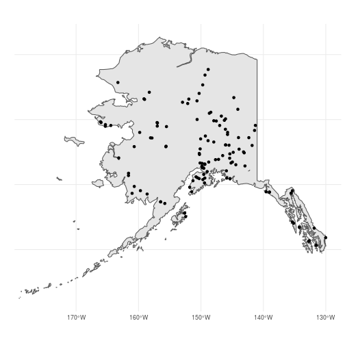
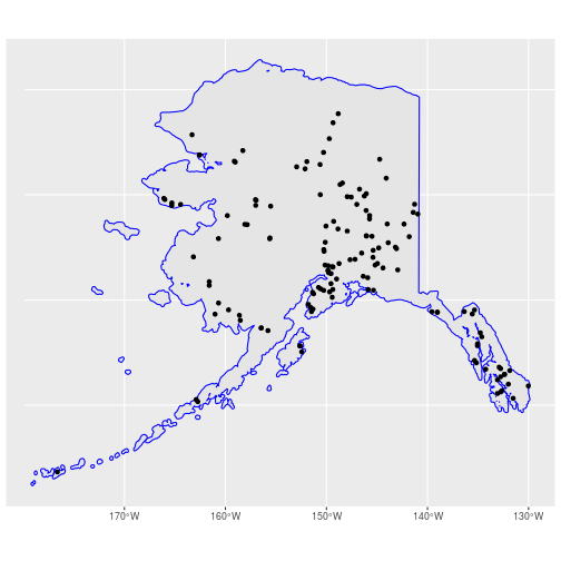
Let’s visualize the output to make sure the filter did what we want. We’ll also recreate the polygon object containing the AK border to give our route map more context (note the use of pipes to avoid creating intermediary objects and the use of st_transform() to set the CRS):
ak <- raster::shapefile("../Spatial_Layers/ak.shp")

ak_sf <- st_as_sf(ak) %>%
  st_transform(crs = 4326)

ggplot() +
  geom_sf(data = ak_sf) +
  geom_sf(data = ak_bbs_sf1) +
  theme_minimal()

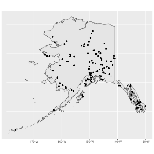
Looks good. Now let’s see the spatial method of doing the same thing. For this, we will use the sf function st_intersection(). This is a predicate function that takes two sf objects (or sfc or sfg objects) and returns the subset of the first object (x) that intersects with the second (y). When x is a point object and y is a polygon, st_intersection() returns the points within the polygon:
ak_bbs_sf2 <- st_intersection(x = bbs_xy_sf, y = ak_sf)

ggplot() +
  geom_sf(data = ak_sf) +
  geom_sf(data = ak_bbs_sf2) +
  theme_minimal()
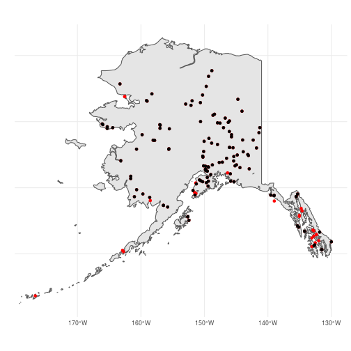
These two methods (filter() vs. st_insection()) should return identical objects so the choice of which to use is up to you. But be careful! In this case, ak_bbs_sf1 and ak_bbs_sf2 are not quite identical because the starting coordinates of somes routes are slightly outside of the ak_sf polygon, likely due to small descrepancies between the two data sets:
shared <- filter(ak_bbs_sf2, routeID %in% ak_bbs_sf1$routeID)

ggplot() +
  geom_sf(data = ak_sf) +
  geom_sf(data = ak_bbs_sf1, color = "red") +
  geom_sf(data = shared) +
  theme_minimal()
Buffering polygons
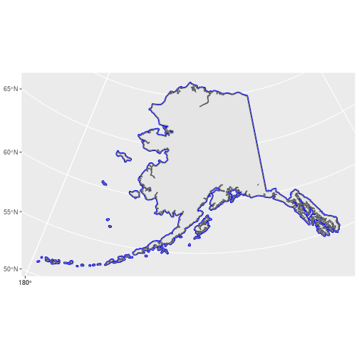
In practice, the difference between the two point objects could a big problem so how can we ensure that all routes fall completely within Alaska? One way is to create a new polygon with boundaries that are outside the ak_sf boundaries and then use st_intersection() to subset the routes within this larger polygon. We can do this in sf using the st_buffer() function. For this function to work properly, we first need to convert the CRS of ak_sf to a projection that uses meters rather than lat/long. We’ll use the Alaska Albers (EPSG = 2964). Next, we add a 25km buffer:
ak_sf2 <- st_transform(ak_sf, crs = 2964)

ak_buffer <- st_buffer(ak_sf2, dist = 25000)

ggplot() +
  geom_sf(data = ak_buffer, color = "blue") +
  geom_sf(data = ak_sf2)
Selecting the BBS routes within this new polygon results in a point object that matches the object we created by filtering:
ak_buffer <- st_transform(ak_buffer, crs = 4326)
ak_bbs_sf <- st_intersection(bbs_xy_sf, ak_buffer)

ggplot() +
  geom_sf(data = ak_sf) +
  geom_sf(data = ak_buffer, color = "blue") +
  geom_sf(data = ak_bbs_sf)
Adding attribute data using joins
Often we may need to add attribute data to spatial objects in order to complete our analyses. We saw in the previous tutorial that we can combine a data.frame object containing attribute data with a sfc object when creating a new sf object. We can also use the dplyr join functions to add attribute data to an existing sf object. To illustrate this, let’s add some count data to the ak_bbs_sf object.
First, read in the count data for a few species:
load("../Spatial_Layers/bbs_counts.rda")
head(bbs_counts)
##   Year  aou speciestotal  routeID
## 1 2006 4860            1 12404002
## 2 1984 4860            2 12404003
## 3 1988 4860            1 12404003
## 4 1995 4860            1 12404003
## 5 1997 4860            1 12404003
## 6 1999 4860            2 12404003
This a slightly-modified version of the raw BBS data. It has been filtered to only contain a subset of years and species (Common raven (aou = 4860), Rusty blackbird (aou = 5090), and Chestnut-backed chickadee (aou = 7410)). In addition, only the total counts (speciestotal) are provided (no stop-level data), and there is a new field called routeID (which is just countrynum, statenum, and Route pasted together to provide a unique ID number for each route).
As before, we only want routes within Alaska. But bbs_counts does not contain spatial data. Luckily, we can add the spatial information AND filter only the Alaska routes at the same time using the dplyr function left_join(). *_join() functions combine the columns of two dataframes (x and y) using a common field(s) to match row attributes. In addition to adding new columns, left_join() only keeps the rows in y that have a matching row in x. So in our case, left_join() uses routeID to add the count data to ak_bbs_sf and drops any routes in bbs_counts that are in not in ak_bbs_sf (i.e., routes that are not in Alaska):
ak_counts_sf <- left_join(ak_bbs_sf, bbs_counts)

## Look at new object
head(ak_counts_sf)
## Simple feature collection with 6 features and 15 fields
## geometry type:  POINT
## dimension:      XY
## bbox:           xmin: -141.2786 ymin: 64.5528 xmax: -141.2786 ymax: 64.5528
## epsg (SRID):    4326
## proj4string:    +proj=longlat +datum=WGS84 +no_defs
##   countrynum statenum Route RouteName Active Stratum BCR LandTypeID
## 1        840        3     1     EAGLE      1      25   4          0
## 2        840        3     1     EAGLE      1      25   4          0
## 3        840        3     1     EAGLE      1      25   4          0
## 4        840        3     1     EAGLE      1      25   4          0
## 5        840        3     1     EAGLE      1      25   4          0
## 6        840        3     1     EAGLE      1      25   4          0
##   RouteTypeID RouteTypeDetailId  routeID FID Year  aou speciestotal
## 1           1                 1 84003001   0 1982 4860            2
## 2           1                 1 84003001   0 1991 4860            2
## 3           1                 1 84003001   0 1992 4860            3
## 4           1                 1 84003001   0 1994 4860            1
## 5           1                 1 84003001   0 1996 4860            2
## 6           1                 1 84003001   0 2001 4860            2
##                    geometry
## 1 POINT (-141.2786 64.5528)
## 2 POINT (-141.2786 64.5528)
## 3 POINT (-141.2786 64.5528)
## 4 POINT (-141.2786 64.5528)
## 5 POINT (-141.2786 64.5528)
## 6 POINT (-141.2786 64.5528)
## Map new object just to make sure it only has the routes we want
ggplot() +
  geom_sf(data = ak_sf) +
  geom_sf(data = ak_counts_sf)
Challenge:
What happens if you useright_join(bbs_counts, ak_bbs_sf) instead of left_join(ak_bbs_sf, bbs_counts)? Hint: what class of object is the first argument in each function and what class of object is the output?
To make our lives easier, let’s also add the species names as new column so we don’t need to refer to species by their AOU code. The dplyr function case_when() makes this easy (look at the help file for more information about the arguments of case_when() and learn how to use it. Without a doubt, case_when() will help you at some point in the future):
ak_counts_sf <- mutate(ak_counts_sf,
                       Species = case_when(aou == 4860 ~ "Common raven",
                                           aou == 5090 ~ "Rusty blackbird",
                                           aou == 7410 ~ "Chestnut-backed chickadee"))
Group level summaries using the tidyverse
The annual BBS counts are necessary in many applications but what if we just want to know, on average, how many individuals of each species are counted on each route? To answer this question, we need to summarise the count data by species AND route. Naive R users may do this by first creating new objects that contain the annual counts of each species at each route, taking the mean count of each of these objects, and then recombining the mean counts into a new data frame. But we’re not naive R users! We know that the tidyverse (specifically dplyr) allows to accomplish exactly those tasks without having to mannually split, summarise, and combine. The dplyr function group_by() creates internal groupings in our original data frame. The summarise() function applies some summary function to each group and returns a dataframe containing the summaries. And since sf objects are data frames, we can use these functions as part of our spatial analysis:
mean_counts_sf <- ak_counts_sf %>%
                group_by(Species, routeID) %>%  # Group by species & route
                 summarise(count = mean(speciestotal)) %>% # Mean count for all years
                  ungroup() # Always ungroup!!!!


head(mean_counts_sf)
## Simple feature collection with 6 features and 3 fields
## geometry type:  POINT
## dimension:      XY
## bbox:           xmin: -136.3619 ymin: 55.32695 xmax: -131.5213 ymax: 59.4505
## epsg (SRID):    4326
## proj4string:    +proj=longlat +datum=WGS84 +no_defs
## # A tibble: 6 x 4
##   Species                    routeID count             geometry
##   <chr>                        <dbl> <dbl>          <POINT [°]>
## 1 Chestnut-backed chickadee 12411139 11     (-136.3619 59.4505)
## 2 Chestnut-backed chickadee 84003020  1    (-134.6278 58.25139)
## 3 Chestnut-backed chickadee 84003021 13.8   (-134.766 58.44237)
## 4 Chestnut-backed chickadee 84003023 13.7  (-133.0848 55.55574)
## 5 Chestnut-backed chickadee 84003024  9.21 (-131.5213 55.32695)
## 6 Chestnut-backed chickadee 84003025  5.17 (-135.5685 59.33637)
As you can see, mean_counts_sf contains the grouping variables (aou & routeID), the newly created summary statistic (count) AND the original sfc column containing the geospatial data for each route! That’s important because we can continue to do spatial analyses or make maps using this new object. For example, let’s look at how mean count varies across the state of Alaska for each species. To do this, we map the size of each point to it’s count (aes(size = count)) and create a separate map (i.e., facet) for each species using facet_wrap(~Species):
## Remove routes that didn't count any of the three species
## These routes will have NA for the count fields
## !is.na() returns only rows that ARE NOT NA
mean_counts_sf <- dplyr::filter(mean_counts_sf, !is.na(Species))

## Recreate AK cities SF object
# Create data.frame with attributes
cities_df <- data.frame(Name = c("Juneau", "Anchorage", "Fairbanks", "Nome"),
                        Population = c(31276, 291826, 3598, 31535),
                        Elevation = c(17, 31, 6, 136))

ju_sfg <- st_point(c(-134.4333, 58.3059)) #Juneau
an_sfg <- st_point(c(-149.8631, 61.2174)) #Anchorage
fa_sfg <- st_point(c(-147.7767, 64.8354)) #Fairbanks
nm_sfg <- st_point(c(-165.4064, 64.5011)) #Nome

cities_sf <- st_sfc(ju_sfg, an_sfg, fa_sfg, nm_sfg, crs = 4326) %>%
               st_sf(cities_df, geometry = .)

ggplot() +
  geom_sf(data = ak_sf) +
  geom_sf(data = cities_sf, color = "red", size = 3) +
  geom_sf(data = mean_counts_sf, aes(size = count),
          show.legend = "point") +
  facet_wrap(~Species) +
  theme_minimal()

So it looks like you have a pretty good chance of seeing Ravens while here in Anchorage, you might be able to see Rusty blackbirds if you’re lucky, but don’t count on getting a Chestnut-backed chickadee without a litte travel. .
Clipping polygons
Based on the map we just created, it seems pretty clear that Rusty blackbirds and Chestnut-backed chickadees prefer different habitats. To examine these differences in a bit more detail, let’s see how these patterns relate to the boundaries of North American “Bird Conservation Regions”. First, let’s download a shapefile containing the boundaries of the 37 BCRs:
download.file(url = "https://www.pwrc.usgs.gov/bba/view/download_map_files/bcr_shp.zip",
              destfile = "../Spatial_Layers/bcr.zip")

unzip(zipfile = "../Spatial_Layers/bcr.zip",
      exdir = "../Spatial_Layers/bcr")

bcr <- raster::shapefile("../Spatial_Layers/bcr/BCR.shp")
Challenge:
What is the class of thebcr object? What function will convert it to a sf object?
### Covert the BCR shapefile to class `sf`
bcr_sf <- st_as_sf(bcr)
If you’d like, you can plot the BCR boundaries using plot(bcr_sf) but be warned it may take several minutes. Since we are interested in learning about the ecosystems in Alaska, let’s clip bcr_sf so that it contains only the BCR’s within the state. In sf, clipping polyons is done using the st_intersection() function that we saw above:
ak_bcr_sf <- st_intersection(ak_sf, bcr_sf)
## Error in geos_op2_geom("intersection", x, y): st_crs(x) == st_crs(y) is not TRUE
Oops, that didn’t work. st_intersection() requires both objects to have the same CRS. So we have to first change the CRS of bcr_sf using st_transform(). For simplicity, we’ll just set crs = st_crs(ak_sf) so that we know bcr_sf will be given the same CRS as ak_sf. Again, we’ll use pipes to do all of these steps at once:
ak_bcr_sf <- st_transform(bcr_sf, crs = st_crs(ak_sf)) %>%
  st_intersection(., ak_sf)
Challenge:
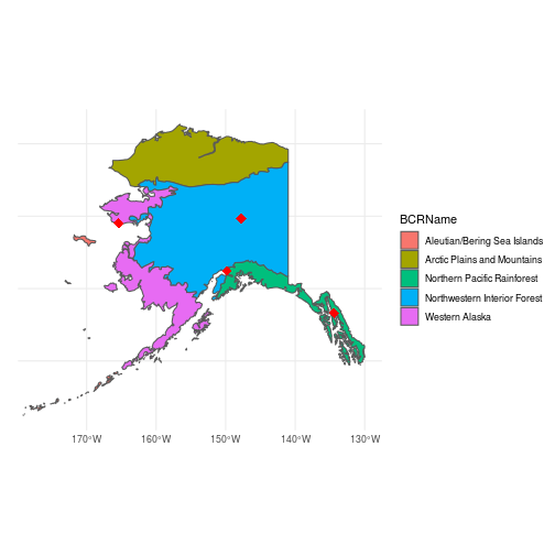
How many different BCRs does Alaska contain? What are their names?Next, let’s make a quick map to visualize the output of st_intersection and make sure it worked correctly:
ggplot() +
  geom_sf(data = ak_bcr_sf, aes(fill = BCRName)) +
  geom_sf(data = cities_sf, shape = 18, color = "red", size = 4) +
  theme_minimal()
Just to illustrate some additional sf functions, let’s compute the area of each BCR using st_area():
st_area(ak_bcr_sf)/100000
## Units: [m^2]
## [1] 3035265.9 7245067.2 2779968.8  103970.9 1412572.7
Without the attribute information (i.e., BCR name), it’s hard to figure out which of the 5 BCRs is actually the biggest. Again, because ak_bcr_sf is a data frame, we can add the areas as a new attribute using the dplyr function mutate(). Because the geometry column contains the spatial information needed to estimate area, we give that as the argument to mutate():
ak_bcr_sf <- dplyr::mutate(ak_bcr_sf, Area = st_area(geometry)/100000)
ak_bcr_sf
## Simple feature collection with 5 features and 4 fields
## geometry type:  GEOMETRY
## dimension:      XY
## bbox:           xmin: -179.1335 ymin: 51.24227 xmax: -129.9795 ymax: 71.35043
## epsg (SRID):    4326
## proj4string:    +proj=longlat +datum=WGS84 +no_defs
##                        BCRName BCRNumber FID
## 1  Arctic Plains and Mountains         3   0
## 2 Northwestern Interior Forest         4   0
## 3               Western Alaska         2   0
## 4  Aleutian/Bering Sea Islands         1   0
## 5  Northern Pacific Rainforest         5   0
##                         geometry            Area
## 1 MULTIPOLYGON (((-166.7441 6... 3035265.9 [m^2]
## 2 GEOMETRYCOLLECTION (LINESTR... 7245067.2 [m^2]
## 3 MULTIPOLYGON (((-162.648 54... 2779968.8 [m^2]
## 4 MULTIPOLYGON (((-179.0905 5...  103970.9 [m^2]
## 5 GEOMETRYCOLLECTION (LINESTR... 1412572.7 [m^2]
Now it’s easier to see that the ‘Northwestern Interior Forest’ BCR is the biggest and the ‘Aleutian/Bering Sea Islands’ is the smallest (within Alaska at least).
Spatial summaries
Now that we have the BCR map, we can layer on the BBS count data to see how the distribution of the three species related to habitat types:
ggplot() +
  geom_sf(data = ak_sf) +
  geom_sf(data = ak_bcr_sf, aes(fill = BCRName),
          show.legend = FALSE) +
  geom_sf(data = cities_sf, color = "red", shape = 18, size = 4) +
  geom_sf(data = mean_counts_sf, aes(size = count),
          show.legend = FALSE) +
  facet_wrap(~Species) +
  theme_minimal()

Ravens appear to be common through all but the Arctic Plains and Mountains BCR, Chestnut-backed chickadees are restricted to the Northern Pacific Rainforest BCR, and Rusty blackbirds occur primarily within the Northwestern Interior Forest BCR.