Introduction to raster data in R

Authors: Michael T. Hallworth
Contributors: Clark S. Rushing

This activity will introduce you to working with raster data in R.

R Skill Level: Intermediate - this activity assumes you have a working knowledge of R

Need to brush up on syntax and data classes in R? See R basics for a refresher.

Objectives & Goals

Upon completion of this activity, you will:

know how to create and write rasters
know how to do basic calculations

Required packages

To complete the following activity you will need the following packages installed: raster sp rgeos

Installing the packages

If installing these packages for the first time consider adding dependencies=TRUE

install.packages("raster",dependencies = TRUE)

install.packages("rgdal",dependencies = TRUE)

install.packages("rgeos",dependencies = TRUE)

install.packages("sp",dependencies = TRUE)

Download R script Last modified: 2019-09-20 18:26:28

What is a raster?

A raster is a spatially explicit matrix or grid where each cell represents a geographic location. Each cell represents a pixel on a surface. The size of each pixel defines the resolution or res of raster. The smaller the pixel size the finer the spatial resolution. The extent or spatial coverage of a raster is defined by the minima and maxima for both x and y coordinates.

Rasters can be created from the following data classes:

Numeric

Integer

Categorical

Raster formats

Raster data are stored in a variety of formats. The table below shows several commonly encountered file types. Use raster::writeFormats() to see the full list.

##      Name                  Long Name File Extension
## 1  raster                   R-raster           .grd
## 5     BIL               Band by Line           .bil
## 8   ascii                  Arc ASCII           .asc
## 22  GTiff                    GeoTIFF          .tiff
## 37 netCDF Network Common Data Format            .nc

Creating & writing rasters

Raster data in R

Let’s begin by creating a raster from scratch. We’ll use the raster package to make an empty raster, set the extent and resolution (res) and assign values. Once we create a raster in R - we’ll take a closer look at the metadata and structure of rasters in R.

load the raster package if you haven’t already done so. If you need to install the raster package - see how to do that here

# load library
library(raster)

Now that the raster library is loaded we can use the raster() function to create a raster in R.

# Create a raster from scratch using raster
firstRaster <- raster(xmn = -100,   # set minimum x coordinate
                      xmx = -60,    # set maximum x coordinate
                      ymn = 25,     # set minimum y coordinate
                      ymx = 50,     # set maximum y coordinate
                      res = c(1,1)) # resolution in c(x,y) direction

Here is what that raster looks like in R

# Take a look at what the raster looks like
firstRaster

## class      : RasterLayer 
## dimensions : 25, 40, 1000  (nrow, ncol, ncell)
## resolution : 1, 1  (x, y)
## extent     : -100, -60, 25, 50  (xmin, xmax, ymin, ymax)
## crs        : +proj=longlat +datum=WGS84 +ellps=WGS84 +towgs84=0,0,0

Notice that the object is of class: RasterLayer has 25 rows, 40 columns and 1000 cells. The resolution (res) is 1x1 degree. The raster’s extent ranges from -100 to -60 degrees longitude and 25 to 50 degrees latitude. The coordinate reference is WGS84 by default because raster recognized our inputs as degrees longitude/latitude. It doesn’t always do so.

Setting raster values

Currently there are no values associated with the raster layer we just created. It’s empty. We can assign values to the raster in a few ways. We’ll set the values of the raster using the [] convention. See the setValues function in the raster package for another way to set values of a raster. We’ll sequence values from 1 to the number of cells within the raster. You can extract the number of cells within a raster using the ncell function.
note - the number of values you supply needs to be equivilant to the number of cells in the raster. You can however provide NA values.

# Assign values to raster 
firstRaster[] <- seq(from = 1, to = ncell(firstRaster),by = 1)

# Take a look at the raster now
firstRaster

## class      : RasterLayer 
## dimensions : 25, 40, 1000  (nrow, ncol, ncell)
## resolution : 1, 1  (x, y)
## extent     : -100, -60, 25, 50  (xmin, xmax, ymin, ymax)
## crs        : +proj=longlat +datum=WGS84 +ellps=WGS84 +towgs84=0,0,0 
## source     : memory
## names      : layer 
## values     : 1, 1000  (min, max)

You should now notice there are a few new attributes to our raster object. We gained data source:, names and values fields. The data source attribute tells us that the raster information is stored in our memory. The names field gave a name to the values we provided. The values we supplied are now contained in the values field.

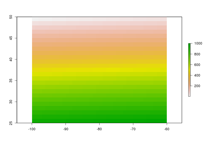
Now that the raster has values we can do a few things - like plot the raster.

plot(firstRaster)

plot of chunk plot-raster-1

Reading rasters from file

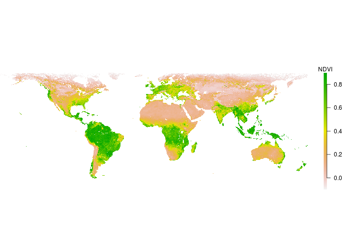
The raster() function within the raster package can also be used to read in a raster from file. Let’s read in some Normalized Difference Vegetation Index (NDVI) data from NASA’s NEO. See where to get data for other potential data sources.

# read in raster layer using raster function
# NDVI <- raster("path/to/raster/file")
NDVI <- raster::raster("../Spatial_Layers/MOD_NDVI_M_2018-01-01_rgb_3600x1800.FLOAT.TIFF")

Let’s take a look at the data

NDVI

## class      : RasterLayer 
## dimensions : 1800, 3600, 6480000  (nrow, ncol, ncell)
## resolution : 0.1, 0.1  (x, y)
## extent     : -180, 180, -90, 90  (xmin, xmax, ymin, ymax)
## crs        : +proj=longlat +datum=WGS84 +no_defs +ellps=WGS84 +towgs84=0,0,0 
## source     : /home/travis/build/mhallwor/mhallwor.github.io/Spatial_Layers/MOD_NDVI_M_2018-01-01_rgb_3600x1800.FLOAT.TIFF 
## names      : MOD_NDVI_M_2018.01.01_rgb_3600x1800.FLOAT

plot of chunk unnamed-chunk-5

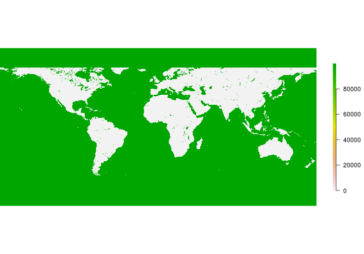
Challenge

Does the NDVI appear as you expected?

If not, why?

What needs to be done to make it fit your expectations?

plot of chunk unnamed-chunk-6