
Generating territories
Contributors: Clark S. Rushing
R Skill Level: Intermediate - this activity assumes you have a working knowledge of R. If you’re not familiar with the apply family of operations in R you may wish to brush up on those before proceeding. See the help files for more information.
Objectives & Goals
Upon completion of this activity, you will:- create territories using kernel density estimates
- create territories using minimum convex polygon
- find the area of each territory
- calculate an index of density
- Extract raster data to terrtiories
Required packages
To complete the following activity you will need the following packages installed: raster sp rgeosInstalling the packages
If installing these packages for the first time consider addingdependencies=TRUE
install.packages("raster",dependencies = TRUE)install.packages("rgdal",dependencies = TRUE)install.packages("rgeos",dependencies = TRUE)install.packages("sp",dependencies = TRUE)Download R script Last modified: 2019-09-20 18:26:28
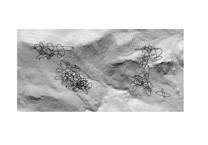
If you work with marked populations or have telemetry-like data you may be interested in constructing territories with either a minimum convex polygon or using kernel density estimation. This activity will illustrate how to go from GPS coordinates of locations for individuals to a territories using both minimum convex polygons and kernel density estimates.
We’ll use location data from a marked population of Ovenbirds breeding at Hubbard Brook Experimental Forest in New Hampshire. The data used in this activity are real data collected in 2012 - we may encounter some hic-cups along the way - we’ll sort them out as/if we encouter them.
library(raster)
library(sp)
library(ks)
Read in bird locations
The location data are stored as a csv file.
OVEN_locs <- read.csv("../Spatial_Layers/OVEN_2012_locs.csv")
## 'data.frame':	1634 obs. of  7 variables:
##  $ Type : Factor w/ 1 level "WAYPOINT": 1 1 1 1 1 1 1 1 1 1 ...
##  $ ident: Factor w/ 551 levels "1","10","100",..: 13 24 494 51 52 53 54 55 56 58 ...
##  $ lat  : num  44 44 44 44 44 ...
##  $ long : num  -71.7 -71.7 -71.7 -71.7 -71.7 ...
##  $ Date : Factor w/ 55 levels "","1-Jun-12",..: 34 34 48 54 54 54 54 54 54 54 ...
##  $ Time : Factor w/ 1566 levels "05:09:30","05:09:36",..: 826 875 112 358 360 372 399 410 428 462 ...
##  $ Bird : Factor w/ 64 levels "__AO","A_KK",..: 1 1 1 1 1 1 1 1 1 1 ...
Convert points to SpatialPoints object
Now that we have the data in R we can create a SpatialPoints object.
# coords = cbind(long,lat)
# crs = WGS84
OVENpts <- sp::SpatialPoints(coords = cbind(OVEN_locs$long,OVEN_locs$lat),
                             proj4string = sp::CRS("+init=epsg:4326"))

# take a peek
head(OVENpts)
## class       : SpatialPoints
## features    : 1
## extent      : -71.74627, -71.74627, 43.95437, 43.95437  (xmin, xmax, ymin, ymax)
## crs         : +init=epsg:4326 +proj=longlat +datum=WGS84 +no_defs +ellps=WGS84 +towgs84=0,0,0
Let’s keep all the data together and make a SpatialPointsDataFrame
OVEN_spdf <- sp::SpatialPointsDataFrame(OVENpts,OVEN_locs)

head(OVEN_spdf)
##       Type ident      lat      long      Date     Time Bird
## 1 WAYPOINT    11 43.95437 -71.74627 26-May-12 09:13:58 __AO
## 2 WAYPOINT    12 43.95435 -71.74624 26-May-12 09:27:42 __AO
## 3 WAYPOINT    95 43.95441 -71.74652  6-Jun-12 06:32:15 __AO
## 4 WAYPOINT   144 43.95450 -71.74707  9-Jun-12 07:23:48 __AO
## 5 WAYPOINT   145 43.95445 -71.74709  9-Jun-12 07:24:17 __AO
## 6 WAYPOINT   146 43.95437 -71.74679  9-Jun-12 07:26:39 __AO
One handy function available in R that isn’t in ArcMap (or at least it wasn’t when I stopped using it) is a function to split a shapefile based on attributes to make a series of spatial layers. The split does exactly that. We’ll use it here to make a SpatialPoints object for each individual in the dataset.
OVEN_sep <- split(x = OVEN_spdf, f = OVEN_spdf$Bird, drop = FALSE)
We now have a list, one element for each unique Bird id. We’ll use this to make our territories.
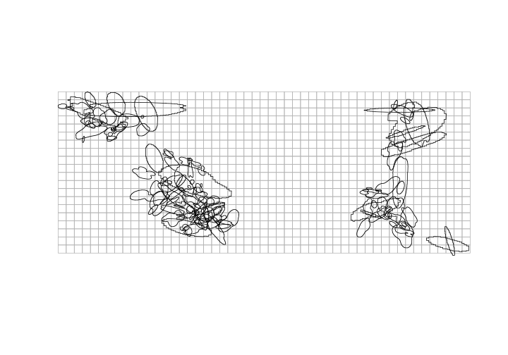
Minimum Convex Hull
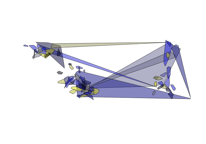
Minimum convex polygon (MCP) generates a polygon that encapsulates all points for an individual. The first step is to make a minimum convex polygon for each individual. The gConvexHull does exactly that. Here we’ll using the lapply function to avoid for loops.
OVENmcp <- lapply(OVEN_sep, FUN = function(x){rgeos::gConvexHull(x)})
The above function returns a list. Ideally, we want all the polygons merged into a single SpatialPolygonsDataFrame. Before we can collapse the list we need to change the ID field in each polygon. Currently, each polygon has the same value in the ID field. Because of that - we can’t combine them. The next bit of code labels each polygon ID field as the Bird id.
OVENmcp <- mapply(OVENmcp, names(OVENmcp),
                  SIMPLIFY = FALSE,
                  FUN = function(x,y){x@polygons[[1]]@ID <- y
                  return(x)})
Now that the ID field is unique for each polygon we can merge the polygons together into a single SpatialPolygons object.
OVENmcp <- do.call(rbind,OVENmcp)
## class       : SpatialPolygons
## features    : 64
## extent      : -71.756, -71.69537, 43.94234, 43.958  (xmin, xmax, ymin, ymax)
## crs         : +init=epsg:4326 +proj=longlat +datum=WGS84 +no_defs +ellps=WGS84 +towgs84=0,0,0
Let’s finish this portion by creating a SpatialPolygonsDataFrame
OVENmcp <- SpatialPolygonsDataFrame(Sr = OVENmcp,
                                    data = data.frame(Bird = names(OVENmcp)),
                                    match.ID = FALSE)
## class       : SpatialPolygonsDataFrame
## features    : 64
## extent      : -71.756, -71.69537, 43.94234, 43.958  (xmin, xmax, ymin, ymax)
## crs         : +init=epsg:4326 +proj=longlat +datum=WGS84 +no_defs +ellps=WGS84 +towgs84=0,0,0
## variables   : 1
## names       : Bird
## min values  : __AO
## max values  : YWAY
There are some issues. Looks like maybe a few points were labeled incorrectly. We’ll come back to fix those up.
Kernel density estimation
Below is just one way to estimate territories using kernel density estimates. We’ll use least-square cross validation to estimate the bandwidth - see Barg et al. 2005 for more information.
First, we’ll estimate the bandwidth for each bird. To do that we’ll use the least-squares cross validation (LSCV) estimator that is part of the ks package. We’ll use lapply again to avoid for loops. The following code will estimate the bandwidth using the coordinates for each bird. LSCV doesn’t like having duplicated points - it may return a warning. Here, we’ll just ignore those warnings for now.
bw <- lapply(OVEN_sep, FUN = function(x){ks::Hlscv(x@coords)})
## Warning in ks::Hlscv(x@coords): Data contain duplicated values: LSCV is not
## well-behaved in this case

## Warning in ks::Hlscv(x@coords): Data contain duplicated values: LSCV is not
## well-behaved in this case
Now that we’ve estimated the bandwidth we can generate the territories. We’ll use the kde (kernel density estimate) in the ks package to create the kernel density estimate. Then in the same function call we’ll convert the kernel density estimate into a raster layer that is spatially explicit. To do this we’ll use the mapply function. See here for more information on what mapply does.
OVEN_kde <-mapply(OVEN_sep,bw,
                  SIMPLIFY = FALSE,
                  FUN = function(x,y){
                   raster(kde(x@coords,h=y))})
Here’s a quick peek at the difference between the MCP and KDE for the same individual.
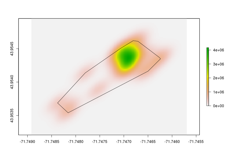
We’re not finished yet with the making the KDE’s. Let’s create a 95% kernel density estimate. To do that we’ll first need to determine what the 95% contour value is. Then, we’ll set all raster values that are less than that value to NA. Once we have the 95% kernel density estimate, we’ll then convert the raster into a polygon so we can find the area, extract landcover data, etc.
Let’s find the 95% contour. To do this we’ll write a custom function. The function will take the kde and probability as inputs. The below function call getContour will make the 95% KDE for us.
# This code makes a custom function called getContour.
# Inputs:
#    kde = kernel density estimate
#    prob = probabily - default is 0.95

getContour <- function(kde, prob = 0.95){
   # set all values 0 to NA
      kde[kde == 0]<-NA
   # create a vector of raster values
      kde_values <- raster::getValues(kde)
   # sort values
      sortedValues <- sort(kde_values[!is.na(kde_values)],decreasing = TRUE)
   # find cumulative sum up to ith location
      sums <- cumsum(as.numeric(sortedValues))
   # binary response is value in the probabily zone or not
      p <- sum(sums <= prob * sums[length(sums)])
   # Set values in raster to 1 or 0
      kdeprob <- raster::setValues(kde, kde_values >= sortedValues[p])
   # return new kde
      return(kdeprob)
}
OVEN_95kde <- lapply(OVEN_kde,
                   FUN = getContour,prob = 0.95)
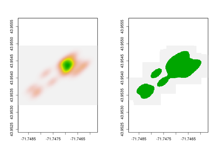
Now that we have the 95% KDE, let’s make a polygon. We’ll use raster’s rasterToPolygons to do that. First, we’ll change all the values in the 95% KDE to 1. After we do that we’ll covert to a polygon. We first convert all values to 1 so that we only make a single polygon that represents the 95% KDE.
OVEN_95poly <- lapply(OVEN_95kde,
                      FUN = function(x){
                        x[x==0]<-NA
                        y <- rasterToPolygons(x, dissolve = TRUE)
                        return(y)
                      })
Before we can merge the 95% KDE together into a single SpatialPolygonsDataFrame we need to change the polygon ID field. We did this above in the MCP example. We’ll use the same processes again here.
OVEN_95poly <- mapply(OVEN_95poly, names(OVEN_95poly),
                  SIMPLIFY = FALSE,
                  FUN = function(x,y){x@polygons[[1]]@ID <- y
                  return(x)})
Now that the ID field is unique for each polygon we can merge the polygons together into a single SpatialPolygons object.
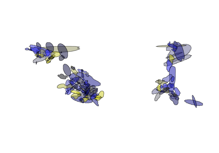
OVEN_95poly <- do.call(rbind,OVEN_95poly)
We’ll finish this portion by adding the bird ID field to the SpatialPolygonsDataFrame. I introduce a new helper function within the sp package called getSpPolygonsIDSlots which does exactly as the function suggests - it returns the ID slot within an object of class SpatialPolygon.
OVEN_95poly$Bird <- getSpPPolygonsIDSlots(OVEN_95poly)
## Warning: use *apply and slot directly
Calculate attributes / Extract raster data
Now that we have made some territories - let’s extract some information. One attribute of interest is territory size. Before we calculate the size, let’s take a look at the crs.
OVEN_95poly
## class       : SpatialPolygonsDataFrame
## features    : 64
## extent      : -71.75641, -71.69242, 43.9414, 43.95862  (xmin, xmax, ymin, ymax)
## crs         : +proj=longlat +datum=WGS84 +ellps=WGS84 +towgs84=0,0,0
## variables   : 2
## names       : layer, Bird
## min values  :     1, __AO
## max values  :     1, YWAY
Notice that the crs is WGS84 or in other words - lat/long, not projected. Let’s first project into a projection that will give us meaningful area estimates. Since these data were gathered at Hubbard Brook Experimental Forest in New Hampshire, let’s use UTM, ZONE 19 N (EPSG:32619) as our projection.
OVENkde_utm <- sp::spTransform(OVEN_95poly, sp::CRS("+init=epsg:32619"))
Now that we have projected data that is in meters we can get a more meaningful measure of area. We’ll use the gArea function in the rgeos package to calculate the area. Let’s have it return the area in hectares.
rgeos::gArea(OVENkde_utm, byid = TRUE)/10000
##       __AO       A_KK       A_MM       APRY       BBAR       BBAW
##  1.0673764  2.4870911  1.8667872  5.0575723  1.9110031  1.0059919
##       BOGA       BRAO       BRAW       BRGA       BWAO       BYAK
##  2.9517315  2.1417197 20.3285926  0.6728364  2.7020183  1.7512344
##       BYWA       GGAR       GRAO       GRAW       GRGA       GWAG
##  2.7786690  5.6030768  3.7193737  1.0639960 14.5445779  4.6073879
##       GYAB       GYAO       KRAG       KROA       KWAG       KYAR
## 35.7228287  1.1734981  1.8457727  4.1336069  0.8192061  9.5846092
##       KYBA       MBAY       MBWA       MM_A       MMAY       MWGA
##  6.2356445  2.1787982  2.8555932  2.5728915  3.6637620  5.0746542
##       OBAK       OKBA       OOYA       ORWA       OWAK   OWOA_MID
##  4.9705965  3.4475742  2.6901538  5.3687464 13.5747309  1.4972174
##       OYAR       PKYA       PPAK       PWKA       PYYA       RBAB
##  0.8822659  4.6840713  5.2457076  3.6238212  1.4511408  0.6944329
##       RGAW       RKAR       ROGA       RWAP       RWKA       RYWA
##  2.5649554 39.4765430 14.8932943  4.5950448  2.2485388  2.6918551
##       WA_Y       WBOA       WGAY       WGGA       WOAW       WOGA
##  4.6116720  1.5454525 21.9530011  2.9143715  1.9042253  2.3967992
##       WORA       WPAB       WWAB       WWAO       YAOY       YBWA
##  2.3690225  5.2167178  3.0969429  3.2959241  6.7857750  4.7502034
##       YKAG       YOAB       YOKA       YWAY
##  2.4014232  1.6383173  2.9426634  3.8435588
Let’s extract some environmental data to our territories. Here, we’ll extract elevation but the process is the same regardless of the variable so long as it’s a raster.
First, we need to read in the digital elevation model (DEM).
# read in raster
DEM <- raster::raster("../Spatial_Layers/hb10mdem.txt")

# project raster to match territories
DEMutm <- projectRaster(DEM, crs = "+init=epsg:32619")
Extract elevation values underlying the territories and append the values to the SpatialPolygonsDataFrame.
OVENkde_utm$meanElev <- extract(DEMutm,OVENkde_utm, mean)
##      BirdID  area_ha Elev_mean Elev_lower Elev_upper
## __AO   __AO 1.067376  742.0644   727.1407   755.8415
## A_KK   A_KK 2.487091  629.2352   617.2643   640.8459
## A_MM   A_MM 1.866787  581.0430   557.9654   591.5341
## APRY   APRY 5.057572  543.4946   523.2714   570.2570
## BBAR   BBAR 1.911003  741.2363   724.1396   777.4179
## BBAW   BBAW 1.005992  780.5575   732.5729   801.6216
Calculate local density metrics
We’ll just scratch the surface here but we’ll compute a basic density metric using the territories we just created. In order to do that we’ll need a raster surface of the area. We can create a basic raster layer using the raster function. Let’s set the res to something spatially meaningful. Below we set it to 100x100m or 1 hectare.
# Empty raster with 1ha resolution
study_plot_raster <- raster::raster(OVENkde_utm, res =c(100,100))

# Covert to SpatialPolygon
study_grid <- as(study_plot_raster,"SpatialPolygons")
For our simple ‘density’ metric let’s figure out how many unique birds use each one hectare grid within the system.
# Create a list with all birds wihtin each 1ha grid cell.
birds_in_ha <- sp::over(study_grid, OVENkde_utm, returnList = TRUE)

# Find how many unique birds are in each cell
study_grid$birds <- unlist(lapply(birds_in_ha,FUN=function(x){length(unique(x$Bird))}))

#convert to raster
birds.per.ha <- rasterize(study_grid,study_plot_raster,study_grid$birds)
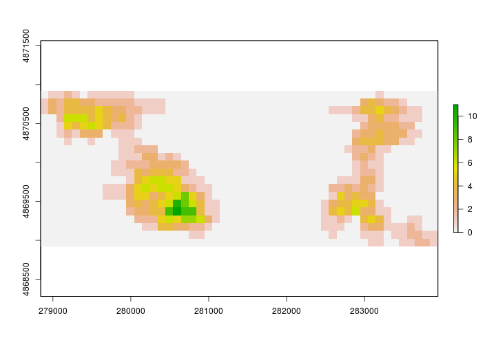
The figure above is a bit misleading. It’s unlikely that there are no Ovenbirds between our study areas.
Challenge:
Take a minute to think about how you may go about removing the areas between our study plots (where we didn't follow individuals). There is more than one way to complete this task. How could you use Spatial Predicates, extract or over to determine which 1 hectare grids were sampled. Perhaps dissolving (gUnion) may be useful.