
Advanced tools for raster data in R
Contributors: Clark S. Rushing
This activity will introduce you more advanced tools to use with raster data in R.
R Skill Level: Intermediate - this activity assumes you have a working knowledge of R
Need to brush up on syntax and data classes in R? See R basics for a refresher.
Objectives & Goals
Upon completion of this activity, you will:- know how to write rasters to file
- know how to deal with raster stack & raster bricks
- know how to work with large rasters
- know how to create raster mosaics
- Be able reclassify rasters
Required packages
To complete the following activity you will need the following packages installed: raster sp rgeosInstalling the packages
If installing these packages for the first time consider addingdependencies=TRUE
install.packages("raster",dependencies = TRUE)install.packages("rgdal",dependencies = TRUE)install.packages("rgeos",dependencies = TRUE)install.packages("sp",dependencies = TRUE)What is a raster?
As a reminder, a raster is a spatially explicit matrix or grid where each cell represents a geographic location. Each cell represents a pixel on a surface. The size of each pixel defines the resolution or res of raster. The smaller the pixel size the finer the spatial resolution. The extent or spatial coverage of a raster is defined by the minima and maxima for both x and y coordinates.
Load the raster package if you haven’t already done so. If you need to install the raster package - see how to do that here
# load library
library(raster)
library(lwgeom)
library(maptools)
library(rgdal)
library(gdalUtils)
Working with large rasters
You can see the details (metadata) of a raster before reading it into R using the GDALinfo function available in the rgdal package. This can be a useful function to get an idea what the data look like, what the CRS is, the resolution and some basic properties like minimum and maximum values.
rgdal::GDALinfo("../Spatial_Layers/MOD_NDVI_M_2018-01-01_rgb_3600x1800.FLOAT.TIFF")
## rows        1800
## columns     3600
## bands       1
## lower left origin.x        -180
## lower left origin.y        -90
## res.x       0.1
## res.y       0.1
## ysign       -1
## oblique.x   0
## oblique.y   0
## driver      GTiff
## projection  +proj=longlat +datum=WGS84 +no_defs
## file        ../Spatial_Layers/MOD_NDVI_M_2018-01-01_rgb_3600x1800.FLOAT.TIFF
## apparent band summary:
##    GDType hasNoDataValue NoDataValue blockSize1 blockSize2
## 1 Float32          FALSE           0        256        256
## apparent band statistics:
##          Bmin       Bmax Bmean Bsd
## 1 -4294967295 4294967295    NA  NA
## Metadata:
## AREA_OR_POINT=Area
## TIFFTAG_RESOLUTIONUNIT=1 (unitless)
## TIFFTAG_XRESOLUTION=1
## TIFFTAG_YRESOLUTION=1
If you use R for spatial processing, sooner or later you’ll need to work with large rasters. By default, when you load a raster into R it loads it into memory. Doing so helps speed up some calculations and ease of access. However, it can limit the size of the rasters you’re able to work with. There are a few work arounds for dealing with large rasters.
The first option is to set the location where the temporary raster is held on your computer. When working with large rasters you may notice that your laptop’s precious hard drive fills up. You can set the location where the raster package stores the temporary files by setting rasterOptions(tmpdir = "/path/to/temp/raster/location"). This can be helpful if you have an external hard drive or drives on your machine that have more space.
raster::rasterOptions(tmpdir = "path/to/drive/with/space")
Another way to deal with processing large rasters is to write them directly to a file rather than returning large rasters into memory. By default rasters are stored in memory, unless they are too large. In which case they are written to a temporary file. Most raster functions accept arguments that are passed directly to the writeRaster function. The additional arguments may include format type, datatype and whether to overwrite the file if it already exists. The default raster format is a .grd file. .grd can be read into R very quickly with the raster package. The downside is there is no driver in GDAL for .grd files so other spatial packages that use GDAL won’t be able to read them. We’ll use this feature in this tutorial.
Raster mosaics
Combining (merging) multiple rasters is usually needed if working with data that spans large geographic extents and you require high resolution raster data. High resolution data like MODIS are saved as tiles. One raster derived from MODIS files you may be familiar with is the treecover dataset. The raster resolution is 30x30m - the global coverage can be over >600 gigabytes.
Moderate Resolution Imaging Spectroradiometer (MODIS) data are stored in tiles. You can see how they’re indexed in the figure below.
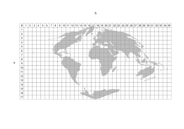
Let’s figure out which tile Arizona falls within. To do that we’ll need to read in the MODIS tile grid pictured above. The MODIS tiles are have a sinusoidal projection.
# Read in MODIS tile grid
MODIStiles <- raster::shapefile("../Spatial_Layers/modis_sinusoidal_grid_world.shp")
Next, we’ll read in a spatial layer for the states, subset out Arizona, and transform to match the MODIStiles.
# Read in states
States <- raster::getData("GADM", country = "United States", level = 1)

# Subset out AZ
AZ <- States[States$NAME_1 == "Arizona",]

# transform AZ to MODIS
AZ_sinsu <- sp::spTransform(AZ, sp::CRS(MODIStiles@proj4string@projargs))
Quick check that the CRS are the same.
identicalCRS(x = MODIStiles, y= AZ_sinsu)
## [1] TRUE
Now that the layers have the same CRS we can use the over function to figure out which MODIS tile/s Arizona falls in.
sp::over(AZ_sinsu,MODIStiles,returnList = TRUE)
## [[1]]
##     cat h v
## 440 441 8 5
## 441 442 9 5
Looks like Arizona spans two MODIS tiles (h08v05 & h09v05). We’ll need to merge those two tiles together later but first we need to know how to read in the data.
We’ll use some MODIS data to derive NDVI values (250m resolution) on March 31st from 2000 to 2017 (MOD09GC). To same some time and bandwith we’ll only read in the values for 2000 and 2017. We’ve provided the links to the other years as well if you’re interested but we’ll only use a select few here.
#MODIS files to download
MODISfiles <- read.csv("../Spatial_Layers/MODIStoget.csv")

# To save space on our hard drive and save time we'll only get year 2000 & 2015
urls_to_get <- paste0("https://ladsweb.modaps.eosdis.nasa.gov",MODISfiles[c(1:2,35:36),2])

# Where to save the files
save_hdf_file <- urls_to_get

# replace url
save_hdf_file <- gsub(x = save_hdf_file,
                      pattern = "https://ladsweb.modaps.eosdis.nasa.gov/archive/allData/6/",
                      replacement = "")
# replace / with .
save_hdf_file <- gsub(x = save_hdf_file,
                     pattern = "[/]",
                     replacement = ".")

# add "../Spatial_Layers/"
save_hdf_file <- paste0("../Spatial_Layers/",save_hdf_file)

# Download using download.file #

mapply(function(x,y){
       download.file(url = x,
                     destfile = y,
                     cacheOK = TRUE,
                     mode = "wb",
                     extra = list(getOption("download.file.extra")))},
       x = urls_to_get,
       y = save_hdf_file)
We’ve gathered MODIS data from h08v05 and h09v05 for 2000 & 2015. Unfortunately, we can’t read the .hdf format directly into a raster using the raster package.
h <- raster::raster(save_hdf_file[1])
Error in .rasterObjectFromFile(x, band = band, objecttype = “RasterLayer”, : Cannot create a RasterLayer >object from this file.
In order to work with MODIS files (*.hdf) we’ll need to first extract the layers (bands) we’re interested in. To do that we’ll use the gdalUtils package.
The sample code below shows how to convert a single .hdf file into a geoTIFF format that we can work with in many different kinds of software.
# Extract the names of the datasets within the compressed hdf file
# Band 1 = Red
# Band 2 = NIR
subsets <- gdalUtils::get_subdatasets(save_hdf_file[1])
We need both red (sur_refl_b01_1) and near infrared (sur_refl_b02_1) bands to generate NDVI values. We’ll extract them from the .hdf files using the gdal_translate function. This function pulls the compressed layer out of the .hdf and creates a new raster in geoTIFF format.
Windows users
#Covert subset of interest into geoTIFF
# red band
gdalUtils::gdal_translate(src_dataset = subsets[2],
                          dst_dataset = "../Spatial_Layers/band_1_2000_h08v05.tiff")
# nir band
gdalUtils::gdal_translate(src_dataset = subsets[3],
                          dst_dataset = "../Spatial_Layers/band_2_2000_h08v05.tiff")
If you have any files or large geographic extents you are working with, running through them all one file at a time would take all day. Let’s have R do tedious task of reading, converting and then processing the .hdf files into geoTIFFs that we can use. We’ll use the mapply function to avoid for loops.
# List the .hdf files
hdf_files <- list.files(path = "../Spatial_Layers/",
                        pattern = "*.hdf",
                        full.names = TRUE)

# generate names of output files
redband_files <- gsub(x = hdf_files,
                  pattern = ".hdf",
                  replacement = "_redband.tiff")

# generate names of output files
nirband_files <- gsub(x = hdf_files,
                  pattern = ".hdf",
                  replacement = "_nirband.tiff")

# note the use of gsub to rename output files
a <- Sys.time()
# Convert all hdf to geoTiff
mapply(a = hdf_files,
       y = redband_files,
       z = nirband_files,
       FUN = function(a,y,z){
       b <- get_subdatasets(a)
       gdal_translate(b[2], dst_dataset = y)
       gdal_translate(b[3], dst_dataset = z)
       })
Sys.time()-a
Linux users
For linux users and possibly MAC users we can skip an intermediate step that working with MODIS on Windows needs to do. Using these operating systems you can read in rasters directly from the object returned using get_subdatasets.
# List the .hdf files
hdf_files <- list.files(path = "../Spatial_Layers/",
                        pattern = "*.hdf",
                        full.names = TRUE)

subsets <- lapply(hdf_files, get_subdatasets)
## List of 4
##  $ : chr [1:8] "HDF4_EOS:EOS_GRID:../Spatial_Layers//MOD09GQ.2000.091.MOD09GQ.A2000091.h08v05.006.2015135231837.hdf:MODIS_Grid_"| __truncated__ "HDF4_EOS:EOS_GRID:../Spatial_Layers//MOD09GQ.2000.091.MOD09GQ.A2000091.h08v05.006.2015135231837.hdf:MODIS_Grid_"| __truncated__ "HDF4_EOS:EOS_GRID:../Spatial_Layers//MOD09GQ.2000.091.MOD09GQ.A2000091.h08v05.006.2015135231837.hdf:MODIS_Grid_"| __truncated__ "HDF4_EOS:EOS_GRID:../Spatial_Layers//MOD09GQ.2000.091.MOD09GQ.A2000091.h08v05.006.2015135231837.hdf:MODIS_Grid_2D:QC_250m_1" ...
##  $ : chr [1:8] "HDF4_EOS:EOS_GRID:../Spatial_Layers//MOD09GQ.2000.091.MOD09GQ.A2000091.h09v05.006.2015135232843.hdf:MODIS_Grid_"| __truncated__ "HDF4_EOS:EOS_GRID:../Spatial_Layers//MOD09GQ.2000.091.MOD09GQ.A2000091.h09v05.006.2015135232843.hdf:MODIS_Grid_"| __truncated__ "HDF4_EOS:EOS_GRID:../Spatial_Layers//MOD09GQ.2000.091.MOD09GQ.A2000091.h09v05.006.2015135232843.hdf:MODIS_Grid_"| __truncated__ "HDF4_EOS:EOS_GRID:../Spatial_Layers//MOD09GQ.2000.091.MOD09GQ.A2000091.h09v05.006.2015135232843.hdf:MODIS_Grid_2D:QC_250m_1" ...
##  $ : chr [1:8] "HDF4_EOS:EOS_GRID:../Spatial_Layers//MOD09GQ.2017.090.MOD09GQ.A2017090.h08v05.006.2017092213051.hdf:MODIS_Grid_"| __truncated__ "HDF4_EOS:EOS_GRID:../Spatial_Layers//MOD09GQ.2017.090.MOD09GQ.A2017090.h08v05.006.2017092213051.hdf:MODIS_Grid_"| __truncated__ "HDF4_EOS:EOS_GRID:../Spatial_Layers//MOD09GQ.2017.090.MOD09GQ.A2017090.h08v05.006.2017092213051.hdf:MODIS_Grid_"| __truncated__ "HDF4_EOS:EOS_GRID:../Spatial_Layers//MOD09GQ.2017.090.MOD09GQ.A2017090.h08v05.006.2017092213051.hdf:MODIS_Grid_2D:QC_250m_1" ...
##  $ : chr [1:8] "HDF4_EOS:EOS_GRID:../Spatial_Layers//MOD09GQ.2017.090.MOD09GQ.A2017090.h09v05.006.2017092213439.hdf:MODIS_Grid_"| __truncated__ "HDF4_EOS:EOS_GRID:../Spatial_Layers//MOD09GQ.2017.090.MOD09GQ.A2017090.h09v05.006.2017092213439.hdf:MODIS_Grid_"| __truncated__ "HDF4_EOS:EOS_GRID:../Spatial_Layers//MOD09GQ.2017.090.MOD09GQ.A2017090.h09v05.006.2017092213439.hdf:MODIS_Grid_"| __truncated__ "HDF4_EOS:EOS_GRID:../Spatial_Layers//MOD09GQ.2017.090.MOD09GQ.A2017090.h09v05.006.2017092213439.hdf:MODIS_Grid_2D:QC_250m_1" ...
# Create empty lists to fill with rasters. This is used to stay consistent with the
# windows workflow.

h08_red_rasters <- h08_nir_rasters <- h09_red_rasters <- h09_nir_rasters <- vector("list",2)

# Use the subsets list to generate rasters
h08_red_rasters[[1]] <- raster(subsets[[1]][2]) #second band of first element
h08_red_rasters[[2]] <- raster(subsets[[3]][2]) #second band of third element

h08_nir_rasters[[1]] <- raster(subsets[[1]][3]) #second band of first element
h08_nir_rasters[[2]] <- raster(subsets[[3]][3]) #second band of third element

h09_red_rasters[[1]] <- raster(subsets[[2]][2]) #second band of first element
h09_red_rasters[[2]] <- raster(subsets[[4]][2]) #second band of third element

h09_nir_rasters[[1]] <- raster(subsets[[2]][3]) #second band of first element
h09_nir_rasters[[2]] <- raster(subsets[[4]][3]) #second band of third element
Now that we’ve created geoTIFF files that we can read into R. Let’s use the output file names (redband_files & nirband_files) we just made to read the rasters back into R. To make it a little easier down the line we’ll make two seperate lists of rasters. The first for h08v05 and the other for h09v05
On Windows
# Note use of grep
h08_red_rasters <- lapply(redband_files[grep(x=redband_files,"h08")],raster)
h08_nir_rasters <- lapply(nirband_files[grep(x=nirband_files,"h08")],raster)

h09_red_rasters <- lapply(redband_files[grep(x=redband_files,"h09")],raster)
h09_nir_rasters <- lapply(nirband_files[grep(x=nirband_files,"h09")],raster)
Now we have two lists that contain rasters. Every raster in h08_rasters has the same extent and resolution. That’s handy because we can create a raster stack. A raster stack is pretty much exactly what it sounds like. A raster stack is two or more stacked (layered) rasters that have the same extent and resolution stored within the same object.
Let’s stack the rasters within each MODIS tile. First the red layers then the near infrared layers. note - the procedures used here may not be the most efficent but were used to illustrate how to use raster stacks / calculations / etc.
h08_rasters <- raster::stack(c(h08_red_rasters,h08_nir_rasters))
h09_rasters <- raster::stack(c(h09_red_rasters,h09_nir_rasters))
h08_rasters
## class      : RasterStack
## dimensions : 4800, 4800, 23040000, 4  (nrow, ncol, ncell, nlayers)
## resolution : 231.6564, 231.6564  (x, y)
## extent     : -11119505, -10007555, 3335852, 4447802  (xmin, xmax, ymin, ymax)
## crs        : +proj=sinu +lon_0=0 +x_0=0 +y_0=0 +a=6371007.181 +b=6371007.181 +units=m +no_defs
## names      : MOD09GQ.2000.091.MOD09GQ.A2000091.h08v05.006.2015135231837.hdf.MODIS_Grid_2D.sur_refl_b01_1, MOD09GQ.2017.090.MOD09GQ.A2017090.h08v05.006.2017092213051.hdf.MODIS_Grid_2D.sur_refl_b01_1, MOD09GQ.2000.091.MOD09GQ.A2000091.h08v05.006.2015135231837.hdf.MODIS_Grid_2D.sur_refl_b02_1, MOD09GQ.2017.090.MOD09GQ.A2017090.h08v05.006.2017092213051.hdf.MODIS_Grid_2D.sur_refl_b02_1
## min values :                                                                                      -32768,                                                                                      -32768,                                                                                      -32768,                                                                                      -32768
## max values :                                                                                       32767,                                                                                       32767,                                                                                       32767,                                                                                       32767
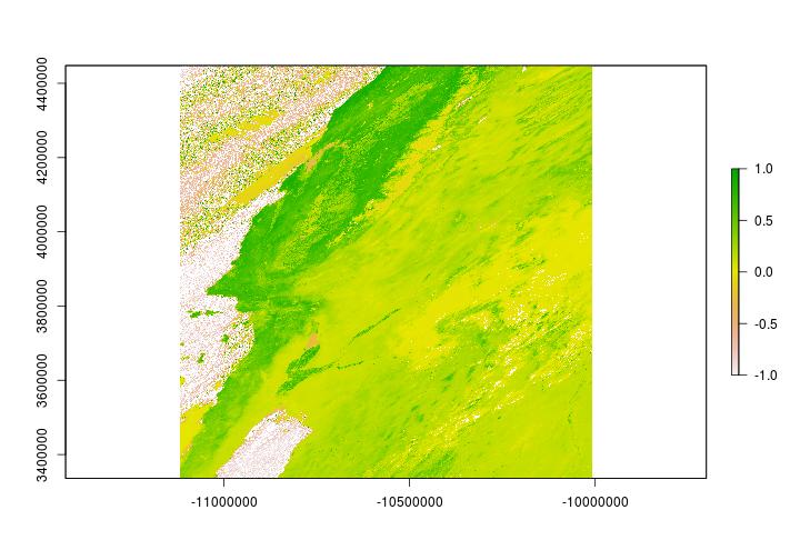
Now that we have all the data required to calculate NDVI - let’s go ahead and do that. We’ll first calculate NDVI within each tile then we’ll merge the two rasters together. That processes is called making a raster mosaic. But first, let’s calculate NDVI. The equation to derive NDVI is as follows:
Raster calculations, for the most part, are pretty intuitive. Below, we’ll create NDVI for each tile separately by indexing the layers (NIR and Red) from with the raster stack.
# Calculate NDVI for each year
h08_NDVI_2000 <- (h08_rasters[[3]]-h08_rasters[[1]])/(h08_rasters[[3]]+h08_rasters[[1]])
h08_NDVI_2017 <- (h08_rasters[[4]]-h08_rasters[[2]])/(h08_rasters[[4]]+h08_rasters[[2]])

# Calculate NDVI for each year
h09_NDVI_2000 <- (h09_rasters[[3]]-h09_rasters[[1]])/(h09_rasters[[3]]+h09_rasters[[1]])
h09_NDVI_2017 <- (h09_rasters[[4]]-h09_rasters[[2]])/(h09_rasters[[4]]+h09_rasters[[2]])
You may notice that some values are -Inf or Inf. We’ll ignore that for now because it doesn’t interfere with our processing. The infinite values occur mostly over water / ocean.
## class      : RasterLayer
## dimensions : 4800, 4800, 23040000  (nrow, ncol, ncell)
## resolution : 231.6564, 231.6564  (x, y)
## extent     : -11119505, -10007555, 3335852, 4447802  (xmin, xmax, ymin, ymax)
## crs        : +proj=sinu +lon_0=0 +x_0=0 +y_0=0 +a=6371007.181 +b=6371007.181 +units=m +no_defs
## source     : /tmp/RtmptVl0SY/raster/r_tmp_2019-09-20_183439_20212_70933.grd
## names      : layer
## values     : -201, 201  (min, max)
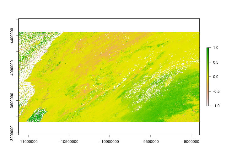
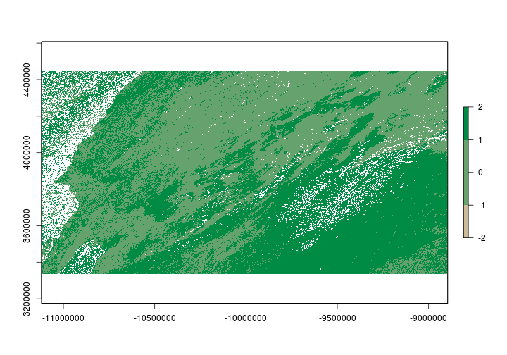
Now that we have NDVI layers for each tile - let’s put them together. The following code will merge the rasters with different spatial extents into a single layer.
# if you haven't already - this is a good
# place to set the tmpdir to store
# large rasters

# rasterOptions(tmpdir = "path/to/temprasters")
a <- Sys.time()
NDVI_2000 <- mosaic(h08_NDVI_2000,
                    h09_NDVI_2000,
                    fun = min,
                    na.rm = TRUE,
                    filename = "../Spatial_Layers/ndvi_2000.tif",
                    overwrite = TRUE)

NDVI_2017 <- mosaic(h08_NDVI_2017,
                    h09_NDVI_2017,
                    fun = min,
                    na.rm = TRUE,
                    filename = "../Spatial_Layers/ndvi_2017.tif",
                    overwrite = TRUE)
Sys.time()-a
## Time difference of 27.56513 secs
NDVI values should range in the values between -1 and 1. Let’s make sure that’s the case by setting the upper and lower values manually.
NDVI_2000[NDVI_2000 > 1] <- NA
NDVI_2000[NDVI_2000 < -1] <- NA

NDVI_2017[NDVI_2017 > 1] <- NA
NDVI_2017[NDVI_2017 < -1] <- NA
Reclassify a raster
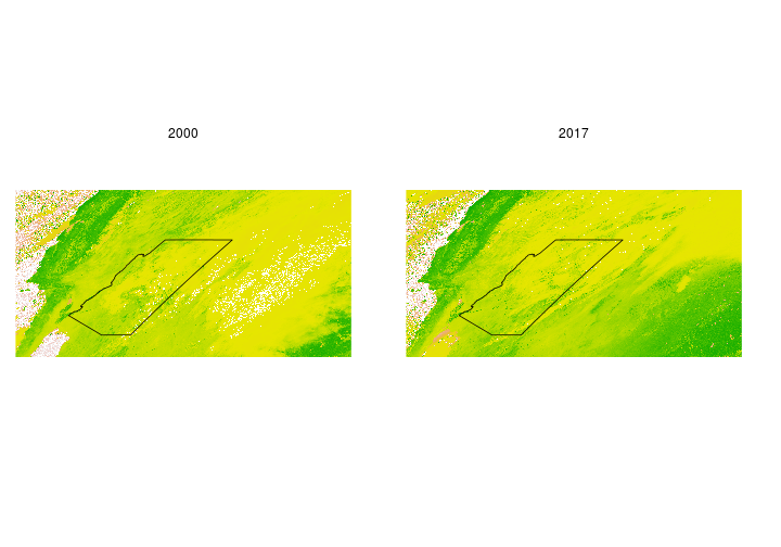
Reclassifying a raster is the process of changing the value of a raster cell based on its current value. Let’s say for example we want to see where on the landscape NDVI differed between 2000 and 2017 on March 31st. We’ll set values to indicate where it was greener and locations where it was less green. First, we’ll need to find the difference in NDVI between the two time periods.
# NDVI in 2017 - NDVI in 2000
diff_ndvi <- NDVI_2017-NDVI_2000
## class      : RasterLayer
## dimensions : 4800, 9600, 46080000  (nrow, ncol, ncell)
## resolution : 231.6564, 231.6564  (x, y)
## extent     : -11119505, -8895604, 3335852, 4447802  (xmin, xmax, ymin, ymax)
## crs        : +proj=sinu +lon_0=0 +x_0=0 +y_0=0 +a=6371007.181 +b=6371007.181 +units=m +no_defs
## source     : /tmp/RtmptVl0SY/raster/r_tmp_2019-09-20_183705_20212_39253.grd
## names      : layer
## values     : -2, 2  (min, max)
## Warning in .hist1(x, maxpixels = maxpixels, main = main, plot = plot, ...):
## 0% of the raster cells were used. 100000 values used.
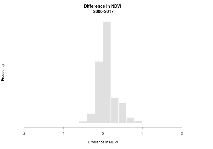
The difference in NDVI ranges from -2 to 2. We’re interested in whether NDVI increased (+) or decreased (-) but we’ll allow for some ‘sampling error’. Let’s say that anywhere between -0.025 and 0.025 is just noise (note: 0.025 was chosen haphazardly and isn’t meaningful we’re just using it for illustration). We can use the reclassify function to set the values for us. The reclassify function requires a matrix that specifies how to reclassify the raster. The matrix consists of rows that have 3 columns. The first column correpsonds to the minimum value that should take the new reclassification value. The second column is the maximum value that will take the reclassification value and the final column contains the new reclassification value.
# from -2 to -0.025 take value 1
# from -0.05 to 0.025 take value 0
# from 0.05 to 2 take value 2
reclassMatrix <- matrix(c(-2,-0.025,1,
                          -0.025,0.025,0,
                          0.025,2,2),3,3,byrow = TRUE)

# reclassify diff_tc to values ranging from 0-2
ndvi_change <- reclassify(diff_ndvi, rcl = reclassMatrix)
Raster brick
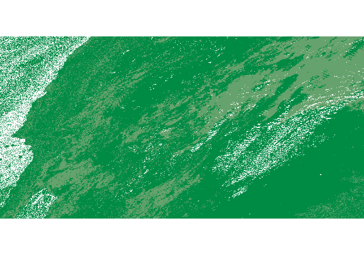
Raster bricks and raster stacks are very similar. One cool thing about raster bricks is that you can make a raster appear the same on any machine. Similar to a template in ArcMap. Let’s convert our ndvi_change layer we just created into a raster brick that contains the RGB (red,green,blue) fields so when you share the raster file with a collaborator it appears the same way it does above. To do that we’ll need to make three copies ndvi_change. Instead of making three copies then adding them into a raster brick. We’ll skip the intermediate step and create a raster brick directly. We’ll reclassify the values directly in the brick.
ndvi_brick <- brick(c(ndvi_change,ndvi_change,ndvi_change))
Now that we have a RasterBrick we’ll reclassify each layer. The first layer will correspond to the red channel, the second layer to the green channel and finally the third layer will correspond to the blue channel. In the plot above I used the colorRampPalette function. We’ll use that again below for consistency.
We’ll need to convert the colors into rgb format.
rgb_vals <- col2rgb(colorRampPalette(c("wheat3","springgreen4"))(3))
##       [,1] [,2] [,3]
## red    205  102    0
## green  186  162  139
## blue   150  109   69
Now let’s reclassify the RasterBrick based on the values.
# Make our reclassify matrix
# note I transposed the rgb_vals

reclassRGB <- cbind(c(-2.5,-0.05,0.05),#from
                    c(-0.05,0.05,2.5),#to
                    t(rgb_vals))#transposed rgb values

ndvi_brick[[1]] <- reclassify(ndvi_brick[[1]],rcl=reclassRGB[,c(1:2,3)])
ndvi_brick[[2]] <- reclassify(ndvi_brick[[2]],rcl=reclassRGB[,c(1:2,4)])
ndvi_brick[[3]] <- reclassify(ndvi_brick[[3]],rcl=reclassRGB[,c(1:2,5)])
Now you can write the RasterBrick to file and send to collaborators and if they read the raster into R using the brick function and plot it using plotRGB is should look exactly the same everytime.
plotRGB(ndvi_brick)
Download R script Last modified: 2019-09-20 18:26:28