Projections

Authors: Michael T. Hallworth
Contributors: Clark S. Rushing

This activity will introduce you projecting spatial data R.

R Skill Level: Intermediate - this activity assumes you have a working knowledge of R

Objectives & Goals

Upon completion of this activity, you will:

• know how and why to project data
• know where to find projection definitions
• know how assign projections
• know how to project spatial data

Required packages

To complete the following activity you will need the following packages installed: raster sp rgeos

Installing the packages

If installing these packages for the first time consider adding dependencies=TRUE

install.packages("raster",dependencies = TRUE)

install.packages("rgdal",dependencies = TRUE)

install.packages("rgeos",dependencies = TRUE)

install.packages("sp",dependencies = TRUE)

---

Download R script Last modified: 2019-09-20 18:26:28

Projections

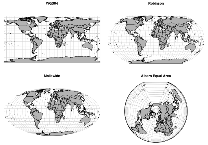
The reason we need projections is so that we can map a three dimensional surface - like the earth in two dimensional space. Unfortunately, not all properties of the 3D surface are maintained when plotting in 2D space. Attributes of the 3D surface such as area, distance, shape and direction are distorted when creating a 2D map. Projections define the way we distort the 3D surface in order to render it in 2D. The projection is the mathmatical equation used to ‘flatten’ the world. Every time we create a map we distort the true surface in some fashion. Different projections preserve different aspects of the 3D properties. Therefore, knowing which projections to use is important when doing spatial analyses. For example, if you’re looking to create a map that looks ‘correct’ a conformal projection might be used as these types of projections preserve shape. If you’re looking to make accurate distance measurements on a surface projections in the equidistant class are appropriate. Take a look at this interactive map that shows different projections - be sure to turn on the distortion ellipse so you can see how distortion changes.

Area of Greenland

Projection	Area
WGS84 (unproj)	661.2549217
Mollewide	214945256.262614
Robinson	345229642.668977
Albers Eq Area	216118436.149343

Projecting data in R isn’t done automatically (for the most part) like it is in ArcMap (on the fly). That means that we need to:

• know the projection of all spatial layers &
• be sure they match

back to top

Finding projection definitions

Each projection has a set of ‘instructions’ on how to distort the earth. For a detailed explaination of each parameter in a coordinate reference system (crs) see proj4.org .

Below are some of my ‘go to’ sites for finding projection definitions.

spatialreference.org

proj4.org

EPSG-registry.org

back to top

Projecting spatial data

The good news is that it’s quite simple to project spatial data in R. First, we need to know whether an object has a coordinate reference system (crs) or not. For the next few examples we’ll use a SpatialPolygonDataFrame that we can get through the raster package.

States <- raster::getData(name = "GADM",
                             country = "United States",
                             level = 1,
                             path = "path/to/save/file",
                             download = TRUE)
# Take a look at the shapefile
States

# Let's remove Alaska and Hawaii for plotting purposes
States <- States[States$NAME_1 != "Alaska" & States$NAME_1 != "Hawaii",]

## class       : SpatialPolygonsDataFrame 
## features    : 52 
## extent      : -179.1506, 179.7734, 18.90986, 72.6875  (xmin, xmax, ymin, ymax)
## crs         : +proj=longlat +datum=WGS84 +no_defs +ellps=WGS84 +towgs84=0,0,0 
## variables   : 13
## names       : OBJECTID, ID_0, ISO,        NAME_0, ID_1,  NAME_1, HASC_1, CCN_1, CCA_1,           TYPE_1,        ENGTYPE_1, NL_NAME_1, VARNAME_1 
## min values  :        1,  244, USA, United States,    1, Alabama,  US.AK,    NA,      , Federal District, Federal District,          , AK|Alaska 
## max values  :       52,  244, USA, United States,   51, Wyoming,  US.WY,    NA,      ,            State,            State,          ,   WY|Wyo.

Access projection of object

You can find the projection information under the coord. ref. field above. To access the coordinate reference system within the object you can do one of the following:

# Use the crs() function in raster
raster::crs(States)

## CRS arguments:
##  +proj=longlat +datum=WGS84 +no_defs +ellps=WGS84 +towgs84=0,0,0

# access the projection slot directly
States@proj4string

## CRS arguments:
##  +proj=longlat +datum=WGS84 +no_defs +ellps=WGS84 +towgs84=0,0,0

# access projection as character 
# - this can be very useful when 
#   using the projection of one
#   object to project another
States@proj4string@projargs

## [1] "+proj=longlat +datum=WGS84 +no_defs +ellps=WGS84 +towgs84=0,0,0"

Projection using sp package

Projecting data in R is very straightforward. The spTransform function found in the sp package makes projecting Spatial objects possible with only a single line of code. Let’s change the projection from WGS84 into North America Lambert Equal Area. See where to find projections for where to find a definition for the North America Lambert Equal Area projection. There are two ways to assign the projection. First is to include a string of the proj4 definition. The second is to refer to the EPSG authority number. Best practice is to use the EPSG code because the database is updated and if changes occur to the projection it will update your map accordingly if you re-run the code. Providing a character string of the projection does will not automatically update unless you manually go back and change the values. One benefit to using a character string (in my opinion) is that it’s easy to manually create new projections with different central maridens that likely aren’t predefined.

# Define the proj4 string 
EqArea <- "+proj=aea 
           +lat_1=20 +lat_2=60 +lat_0=40 +lon_0=-96 +x_0=0 +y_0=0 
           +ellps=GRS80 
           +datum=NAD83 
           +units=m +no_defs"

# project using the string
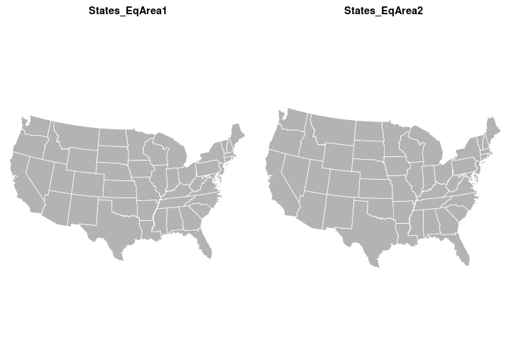
States_EqArea2 <- sp::spTransform(x = States,
                                 CRSobj = CRS(EqArea))

# project using the ESPG authority number
States_EqArea1 <- sp::spTransform(x = States,
                                 CRS("+init=epsg:5070"))

Let’s remove the coordinate reference system (crs) from States then try to project it and see what happens.

crs(States)<-NA
States

## class       : SpatialPolygonsDataFrame 
## features    : 49 
## extent      : -124.7628, -66.94889, 24.52042, 49.3833  (xmin, xmax, ymin, ymax)
## crs         : NA 
## variables   : 13
## names       : OBJECTID, ID_0, ISO,        NAME_0, ID_1,  NAME_1, HASC_1, CCN_1, CCA_1,           TYPE_1,        ENGTYPE_1, NL_NAME_1, VARNAME_1 
## min values  :        1,  244, USA, United States,    1, Alabama,  US.AL,    NA,      , Federal District, Federal District,          ,   AL|Ala. 
## max values  :       52,  244, USA, United States,   51, Wyoming,  US.WY,    NA,      ,            State,            State,          ,   WY|Wyo.

Defining projection to SpatialObject

If your SpatialObject doesn’t have a coordinate reference system (crs) defined it won’t know how to project the data. Therefore, if the coordinate reference system (crs) is NA you need to assign it. A word of caution - R will let you assign any valid PROJ.4 CRS string as the coordinate reference system to an object even if it doesn’t make sense.

# Let's take a look at the extent of the 
# shapefile to give us a clue to what projection
# it may be. 
States

## class       : SpatialPolygonsDataFrame 
## features    : 49 
## extent      : -124.7628, -66.94889, 24.52042, 49.3833  (xmin, xmax, ymin, ymax)
## crs         : NA 
## variables   : 13
## names       : OBJECTID, ID_0, ISO,        NAME_0, ID_1,  NAME_1, HASC_1, CCN_1, CCA_1,           TYPE_1,        ENGTYPE_1, NL_NAME_1, VARNAME_1 
## min values  :        1,  244, USA, United States,    1, Alabama,  US.AL,    NA,      , Federal District, Federal District,          ,   AL|Ala. 
## max values  :       52,  244, USA, United States,   51, Wyoming,  US.WY,    NA,      ,            State,            State,          ,   WY|Wyo.

The States object appears to have a +proj=longlat since the extent of the object is in degrees longitude, latitude. Below we’ll assign the WGS84 projection.

# Define WGS84 in proj4 string format
WGS84 <- "+proj=longlat +datum=WGS84 
          +no_defs +ellps=WGS84 +towgs84=0,0,0"

# use the crs() function in the raster package
# to define the projection
crs(States) <- WGS84

# take a look
States

## class       : SpatialPolygonsDataFrame 
## features    : 49 
## extent      : -124.7628, -66.94889, 24.52042, 49.3833  (xmin, xmax, ymin, ymax)
## crs         : +proj=longlat +datum=WGS84 +no_defs +ellps=WGS84 +towgs84=0,0,0 
## variables   : 13
## names       : OBJECTID, ID_0, ISO,        NAME_0, ID_1,  NAME_1, HASC_1, CCN_1, CCA_1,           TYPE_1,        ENGTYPE_1, NL_NAME_1, VARNAME_1 
## min values  :        1,  244, USA, United States,    1, Alabama,  US.AL,    NA,      , Federal District, Federal District,          ,   AL|Ala. 
## max values  :       52,  244, USA, United States,   51, Wyoming,  US.WY,    NA,      ,            State,            State,          ,   WY|Wyo.

back to top

Projecting Rasters

Word of caution: Consider the following when using raster data for analyses. In general it’s not the best approach to project rasters. Below is a brief description for why it’s not a great idea to project rasters. The text below is borrowed heavily from rspatial.org, a blog written by Robert Hijmans - the author of the raster package. Vector data can be transformed to and from different projections without losing precision. However, that is not true with raster data. Because rasters consist of rectangular cells that are the same size with respect to the CRS units, their actual size may vary. It’s not possible to transform a raster cell by cell. Therefore, estimates for the values of new cells are made based on the values in the old cells. A commonly used approach to estimating the values of the new cells is ‘nearest neighbor’. Otherwise an interpolation (e.g. ‘bilinear’) approach is used - this can be set by the user when projecting rasters using the projectRaster function. Because projecting rasters affects cell values, in most cases you will want to avoid projecting raster data and project SpatialObjects instead.

For mapping purposes we’ll go over how to project rasters.

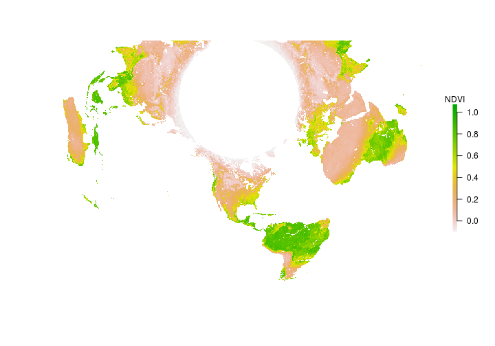
Let’s grab a raster we are already familiar with. We’ll use the NDVI raster from January 2018.

# read in raster layer using raster function
# NDVI <- raster("path/to/raster/file")
NDVI <- raster::raster("../Spatial_Layers/MOD_NDVI_M_2018-01-01_rgb_3600x1800.FLOAT.TIFF")

## class      : RasterLayer 
## dimensions : 1800, 3600, 6480000  (nrow, ncol, ncell)
## resolution : 0.1, 0.1  (x, y)
## extent     : -180, 180, -90, 90  (xmin, xmax, ymin, ymax)
## crs        : +proj=longlat +datum=WGS84 +no_defs +ellps=WGS84 +towgs84=0,0,0 
## source     : /home/travis/build/mhallwor/mhallwor.github.io/Spatial_Layers/MOD_NDVI_M_2018-01-01_rgb_3600x1800.FLOAT.TIFF 
## names      : MOD_NDVI_M_2018.01.01_rgb_3600x1800.FLOAT

The NDVI raster is pretty large. It has 6480000 cells. It takes a little while to project the raster.

a <- Sys.time()
NDVIproj <- raster::projectRaster(from = NDVI,
                          crs = sp::CRS("+init=epsg:5070"))
Sys.time()-a

## class      : RasterLayer 
## dimensions : 4332, 4922, 21322104  (nrow, ncol, ncell)
## resolution : 6880, 5060  (x, y)
## extent     : -16935118, 16928242, -7001394, 14918526  (xmin, xmax, ymin, ymax)
## crs        : +proj=aea +lat_1=29.5 +lat_2=45.5 +lat_0=23 +lon_0=-96 +x_0=0 +y_0=0 +ellps=GRS80 +towgs84=0,0,0,0,0,0,0 +units=m +no_defs 
## source     : /home/travis/build/mhallwor/mhallwor.github.io/Spatial_Layers/MOD_NDVI_M_2018-01-01_rgb_3600x1800.FLOAT_proj.tif 
## names      : MOD_NDVI_M_2018.01.01_rgb_3600x1800.FLOAT_proj 
## values     : -5.768277, 100005.5  (min, max)

On your own:

Compare the number of cells raster::ncell(raster) before and after projecting the raster. Are they the same or are they different? If they're different, why do you think they differ?

back to top