Extracting raster data
Contributors: Clark S. Rushing
R Skill Level: Intermediate - this activity assumes you have a working knowledge of R
This activity incorporates the skills learned in the Points, Polygons, Raster & Projections activities.
Objectives & Goals
Upon completion of this activity, you will:- know how to extract raster data to spatial layers
- know how to summarize extracted data
Required packages
To complete the following activity you will need the following packages installed: raster velox sp rgeosInstalling the packages
If installing these packages for the first time consider addingdependencies=TRUE
install.packages("raster")
install.packages("velox")
install.packages("sp")
install.packages("rgeos")
Download R script Last modified: 2019-09-20 18:26:28
library(raster)
library(velox)
library(sp)
library(rgeos)
Extracting raster data to an area or location of interest is a common GIS task. There are a few things to keep in mind while extracting raster data in R. First, as we’ve seen in Projections it’s best to use projected data. Second, make sure the two layers have the same coordinate reference system. Lastly, make sure you know the data class you’re extracting (i.e., continuous, factor, etc.)
Extracting Raster to SpatialPoints
Extracting raster data to SpatialLayers can be done using the extract function in the raster package. See extract function documentation for details regarding options.
Gathering spatial data
For this first example, we’ll use a digital elevation model (DEM) of Hubbard Brook Experimental Forest in New Hampshire. The dem is of class numerical. Which means we can perform numerical calculations like finding the mean and range of the data. Below, we’ll use a data set where the data are factors.
Reading in the DEM
# read in DEM of HBEF
DEM <- raster::raster("../Spatial_Layers/hb10mdem.txt")
Each summer, the Smithsonian Conservation Biology Institute’s Migratory Bird Center conducts point counts at nearly 400 locations throughout Hubbard Brook. The point count locations have been georeferenced. Let’s extract the elevation of each survey location. First, we’ll need to read in the in the survey locations.
SurveyLocs <- raster::shapefile("../Spatial_Layers/hbef_valleywideplots.shp")
## class       : SpatialPointsDataFrame
## features    : 395
## extent      : 275500, 283000, 4866300, 4871200  (xmin, xmax, ymin, ymax)
## crs         : +proj=utm +zone=19 +datum=NAD83 +units=m +no_defs +ellps=GRS80 +towgs84=0,0,0
## variables   : 4
## names       : X8.digit.Pl, Plot.Tag, UTM.Eastin, UTM.Northi
## min values  :    75567500,        1,     275500,    4866300
## max values  :    83070200,       99,     283000,    4871200
Before we proceed, let’s make sure the CRS is the same in for both the raster layer (DEM) and the SpatialPoints layer.
crs(SurveyLocs)
## CRS arguments:
##  +proj=utm +zone=19 +datum=NAD83 +units=m +no_defs +ellps=GRS80
## +towgs84=0,0,0
crs(DEM)
## CRS arguments:
##  +proj=longlat +datum=WGS84 +no_defs +ellps=WGS84 +towgs84=0,0,0
The two layers have different coordinate reference systems. We’ll need to transform the SpatialPoints layer to match the raster (DEM). See caution projecting rasters for details on why we’ll project the SpatialPoints instead of the raster.
# Transform points to match CRS of the DEM
SurveyLocs_proj <- sp::spTransform(x = SurveyLocs,
                                   CRSobj = crs(DEM))
Now that the two layers have the same CRS we can extract the elevation to survey points. We’ll use the extract function available in the raster package. The first argument is the raster values you want to extract. The second argument (y) can be a SpatialObject or matrix.
# Extract elevation to SpatialPoints
surveyElev <- raster::extract(x = DEM,
                              y = SurveyLocs_proj)
The resulting object is a vector with the same length as SurveyLocs_proj.
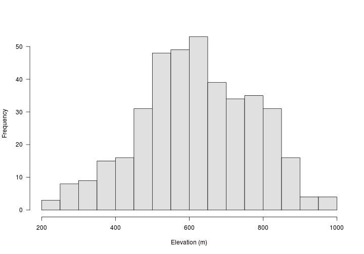
## num [1:395] 475 494 555 588 575 574 574 588 602 630 ...
We can add the data directly into the SpatialPointsDataFrame with the following code.
SurveyLocs_proj$Elev_m <- raster::extract(x = DEM,
                                          y = SurveyLocs_proj)
## class       : SpatialPointsDataFrame
## features    : 395
## extent      : -71.79809, -71.70358, 43.91606, 43.95997  (xmin, xmax, ymin, ymax)
## crs         : +proj=longlat +datum=WGS84 +no_defs +ellps=WGS84 +towgs84=0,0,0
## variables   : 5
## names       : X8.digit.Pl, Plot.Tag, UTM.Eastin, UTM.Northi, Elev_m
## min values  :    75567500,        1,     275500,    4866300,    240
## max values  :    83070200,       99,     283000,    4871200,    965

Extract raster to polygon/s
Below, we’ll determine the proportion of landcover types within Alaska. In order to complete this task, some new functions will be introduced but we’ll also use some skills we learned in other activities.
Gathering spatial data
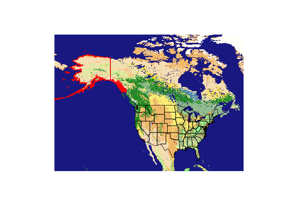
We’re interested in quantifying landcover around Anchorage, AK or more broadly the landcover types found in Alaska.
First, we’ll read in the landcover classes. In this example, we’ll use landcover data with a relatively coarse resolution for simplicity and speed.
# Read in landcover data
LandCover <- raster::raster("../Spatial_Layers/MCD12C1_T1_2011-01-01_rgb_3600x1800.TIFF")
## class      : RasterLayer
## dimensions : 1800, 3600, 6480000  (nrow, ncol, ncell)
## resolution : 0.1, 0.1  (x, y)
## extent     : -180, 180, -90, 90  (xmin, xmax, ymin, ymax)
## crs        : +proj=longlat +datum=WGS84 +no_defs +ellps=WGS84 +towgs84=0,0,0
## source     : /home/travis/build/mhallwor/mhallwor.github.io/Spatial_Layers/MCD12C1_T1_2011-01-01_rgb_3600x1800.TIFF
## names      : MCD12C1_T1_2011.01.01_rgb_3600x1800
## values     : 0, 255  (min, max)
| Code | Land Cover Class |
|---|---|
| 01 | Evergreen Needleleaf forest |
| 02 | Evergreen Broadleaf forest |
| 03 | Deciduous Needleleaf forest |
| 04 | Deciduous Broadleaf forest |
| 05 | Mixed forest |
| 06 | Closed shrublands |
| 07 | Open shrublands |
| 08 | Woody savannas |
| 09 | Savannas |
| 10 | Grasslands |
| 11 | Permanent wetlands |
| 12 | Croplands |
| 13 | Urban and built-up |
| 14 | Cropland/Natural vegetation mosaic |
| 15 | Snow and ice |
| 16 | Barren or sparsely vegetated |
| 17 | Water bodies |
| 18 | Tundra |
*National Center for Atmospheric Research Staff (Eds). Last modified 10 Feb 2017. “The Climate Data Guide: CERES: IGBP Land Classification.” Retrieved from https://climatedataguide.ucar.edu/climate-data/ceres-igbp-land-classification.
Now that we have a basic Landcover layer, we’ll can gather spatial data for Alaska. We’ll grab the entire United States and then subset out Alaska.
States <- raster::getData("GADM", country = "United States", level = 1)
AK <- States[States$NAME_1=="Alaska",]
## class       : SpatialPolygonsDataFrame
## features    : 1
## extent      : -179.1506, 179.7734, 51.20972, 72.6875  (xmin, xmax, ymin, ymax)
## crs         : +proj=longlat +datum=WGS84 +no_defs +ellps=WGS84 +towgs84=0,0,0
## variables   : 10
## names       : GID_0,        NAME_0,   GID_1, NAME_1, VARNAME_1, NL_NAME_1, TYPE_1, ENGTYPE_1, CC_1, HASC_1
## value       :   USA, United States, USA.2_1, Alaska, AK|Alaska,        NA,  State,     State,   NA,  US.AK
Great - now we have a SpatialPolygonsDataFrame of Alaska. Take note of the CRS.
Landcover types are factors since they’re categorical. The reason that’s important is because when extracting raster data there are options to apply a function to the underlying raster data. For example, the extract function allows users to specify a function like mean and the function will return the mean raster value under the area of interest. However, because landcover types are factors, returning the mean landcover type is meaningless. Instead, as a final result were interested in having a table giving the percent of each landcover type in Alaska. We’ll work our way up to that. We’ll start by first extracting the landcover types in Alaska using the extract function available in the raster package.
The velox package is much faster for extracting raster values, especially with large data sets. See what else velox can do velox documentation
# Extract using the raster package

# x = raster layer
# y = SpatialLayer

a <- Sys.time()
AK_lc <- extract(x = LandCover,
                 y = AK)
Sys.time()-a
## Time difference of 2.391696 mins
# Extract using velox
LandCover_velox <- velox::velox(LandCover)

b <- Sys.time()
AK_lc_velox <- LandCover_velox$extract(AK)
Sys.time() - b
## Time difference of 25.34263 secs
On your own:
What does theextract function return? How are the data stored? How do you think the resulting object would differ if we had more than one SpatialPolygon?
## List of 1
##  $ : num [1:27934] NA 10 10 10 10 10 10 10 10 10 ...
The extract function returns a list with the raster values that fall within our area of interest. Let’s summarize the data a little bit. We’ll use the table function to briefly summarize the landcover types within Alaska.
table(AK_lc)
## AK_lc
##     1     3     4     5     7     8     9    10    11    13    14    15
##   877     5     3   426 13745  6333    59  4264    25     2     5  1349
##    16
##     6

Custom function to summarize landcover data
Let’s write a simple function that returns the landcover data as a percentage. The first thing we’ll do is make a sorted vector that has all the unique landcover types that are found in the landcover data set.
# sort the unique values in LandCover
z <- sort(unique(raster::values(LandCover)))
## [1] 1 2 3 4 5 6 7 8 9 10 11 12 13 14 15 16
Now that we have a sorted vector of all the landcover types in the LandCover raster - let’s summarize the landcover types in Alaska. To do that we’ll need to write a custom function. Our function will be called summarizeLC. The summarizeLC function will except three arguments: x = extracted landcover data, LC_classes = land cover classes in the data set & LC_names a vector that contains the names of the landcover types. We’ll set LC_names = NULL so it’s optional.
summarizeLC <- function(x,LC_classes,LC_names = NULL){
               # Find the number of cells
               y <- length(x)
               # Make a table of the cells
               tx <- table(x)
               # Create an empty array to store landcover data
               LC <- array(NA,c(1,length(LC_classes)))
               # Loop through the landcover types & return
               # the number of cells within each landcover type
               for(i in seq(LC_classes)){
               LC[1,i] <- ifelse(LC_classes[i] %in% dimnames(tx)[[1]],
                                 #if true
                                 tx[which(dimnames(tx)[[1]]==LC_classes[i])],
                                 # if false
                                 0)
               } # end loop
               # Convert to percentage
               LC <- LC/y
               #
               if(!is.null(LC_names)){
                 colnames(LC)<-LC_names}
               else{colnames(LC)<-LC_classes}

               return(LC)
}
Here we’ll apply our function to the extracted raster data. Remember, the extracted raster data (AZ_lc) are stored as a list. Because of that we’ll use the lapply function to apply our function (summarizeLC) to all elements of a list. This is especially useful when you extract raster values to more than one polygon, as the extracted values are stored in separate lists.
summaryValues <- lapply(AK_lc,FUN = summarizeLC,LC_classes = z)
Here is what the final result may look like.
##                                    Percent
## Evergreen Needleleaf forest          0.031
## Evergreen Broadleaf forest           0.000
## Deciduous Needleleaf forest          0.000
## Deciduous Broadleaf forest           0.000
## Mixed forest                         0.015
## Closed shrublands                    0.000
## Open shrublands                      0.492
## Woody savannas                       0.227
## Savannas                             0.002
## Grasslands                           0.153
## Permanent wetlands                   0.001
## Croplands                            0.000
## Urban and built-up                   0.000
## Cropland/Natural vegetation mosaic   0.000
## Snow and ice                         0.048
## Barren or sparsely vegetated         0.000
On your own:
Find the proportion of each landcover type within your state. Use theextract function and the custom summarizeLC function return the landcover percentages.
Challenge:
Compare and contrast the landcover classes for two or more states.## New Hampshire West Virginia
## Deciduous Broadleaf forest 0.111 0.905
## Mixed forest 0.867 0.012
## Grasslands 0.000 0.002
## Urban and built-up 0.011 0.003
## Cropland/Natural vegetation mosaic 0.004 0.078
