Introduction to spatial polygons in R

Authors: Michael T. Hallworth
Contributors: Clark S. Rushing

This activity will introduce you to working with spatial polygons in R.

R Skill Level: Intermediate - this activity assumes you have a working knowledge of R

Objectives & Goals

Upon completion of this activity, you will:

know how to create and write spatial polygons
Be able to project spatial polygons
Be able to dissolve boundaries

Required packages

To complete the following activity you will need the following packages installed: raster sp rgeos

Installing the packages

If installing these packages for the first time consider adding dependencies=TRUE

install.packages("raster",dependencies = TRUE)

install.packages("rgdal",dependencies = TRUE)

install.packages("rgeos",dependencies = TRUE)

install.packages("sp",dependencies = TRUE)

Download R script Last modified: 2019-09-20 18:26:28

What are spatial polygons?

Spatial polygons are a set of spatially explicit shapes/polygons that represent a geographic location. Spatial polygons are composed of vertices which are a set of a series of x and y coordinates or Spatial points. Spatial polygons can be combined with data frames to create what’s called a SpatialPolygonsDataFrame. The difference between SpatialPolygons and SpatialPolygonsDataFrame are the attributes that are associated with the polygons. SpatialPolygonsDataFrames have additional information associated with the polygon (e.g., site, year, individual, etc.) while SpatialPolygons contain only the spatial information (vertices) about the polygon.

Creating & writing spatial polygons

Spatial Polygons in R

Let’s begin by creating a set spatial polygons layer from scratch. We’ll use the sp package to make a SpatialPolygons object. First we need to create a set of XY coordinates that represent the vertices of a polygon. We’ll use use some randomly generated XY coordinates. Once we create a SpatialPolygons object in R - we’ll take a closer look at its metadata and structure.

load the sp package if you haven’t already done so. If you need to install the sp package - see how to do that here

# load library
library(sp)

Now that the sp library is loaded we can use the SpatialPolygons() function to create a SpatialPolygons object in R.

Here is the general workflow for generating polygons from scratch:

Determine a set of coordinates for the vertices

note that the first and last vertex need to be the same to 'close' the polygon.

Give the polygon an ID

# Make a set of coordinates that represent vertices
# with longitude and latitude in the familiar
# degrees

x_coords <- c(-60,-60,-62,-62,-60)
y_coords <- c(20,25,25,20,20)

Next we use the Polygon function in the sp package to make a polygon from our matrix of vertices

poly1 <- sp::Polygon(cbind(x_coords,y_coords))

Then we make poly1 into a Polygon class using the Polygons function

firstPoly <- sp::Polygons(list(poly1), ID = "A")

str(firstPoly,1)

## Formal class 'Polygons' [package "sp"] with 5 slots

Then we can make firstPoly into a SpatialPolygons

firstSpatialPoly <- sp::SpatialPolygons(list(firstPoly))

firstSpatialPoly

## An object of class "SpatialPolygons"
## Slot "polygons":
## [[1]]
## An object of class "Polygons"
## Slot "Polygons":
## [[1]]
## An object of class "Polygon"
## Slot "labpt":
## [1] -61.0  22.5
## 
## Slot "area":
## [1] 10
## 
## Slot "hole":
## [1] FALSE
## 
## Slot "ringDir":
## [1] 1
## 
## Slot "coords":
##      x_coords y_coords
## [1,]      -60       20
## [2,]      -62       20
## [3,]      -62       25
## [4,]      -60       25
## [5,]      -60       20
## 
## 
## 
## Slot "plotOrder":
## [1] 1
## 
## Slot "labpt":
## [1] -61.0  22.5
## 
## Slot "ID":
## [1] "A"
## 
## Slot "area":
## [1] 10
## 
## 
## 
## Slot "plotOrder":
## [1] 1
## 
## Slot "bbox":
##   min max
## x -62 -60
## y  20  25
## 
## Slot "proj4string":
## CRS arguments: NA

We can create two or more polygons into a single SpatialPolygon file as well. That workflow looks something like this:

# define the vertices
x1 <- c(-60,-60,-62,-62,-60)
x2 <-c(-50,-50,-55,-55,-50)
y1 <- c(20,25,25,20,20)
y2 <- c(15,25,25,15,15)

# assign the vertices to a `polygon` 
poly1 <- sp::Polygon(cbind(x1,y1))
poly2 <- sp::Polygon(cbind(x2,y2))

# This step combines the last two together - making Polygons and then SpatialPolygons
TwoPolys <- sp::SpatialPolygons(list(sp::Polygons(list(poly1),ID = "A"),
                                     sp::Polygons(list(poly2), ID = "B")))

#Let's take a look
TwoPolys

## An object of class "SpatialPolygons"
## Slot "polygons":
## [[1]]
## An object of class "Polygons"
## Slot "Polygons":
## [[1]]
## An object of class "Polygon"
## Slot "labpt":
## [1] -61.0  22.5
## 
## Slot "area":
## [1] 10
## 
## Slot "hole":
## [1] FALSE
## 
## Slot "ringDir":
## [1] 1
## 
## Slot "coords":
##       x1 y1
## [1,] -60 20
## [2,] -62 20
## [3,] -62 25
## [4,] -60 25
## [5,] -60 20
## 
## 
## 
## Slot "plotOrder":
## [1] 1
## 
## Slot "labpt":
## [1] -61.0  22.5
## 
## Slot "ID":
## [1] "A"
## 
## Slot "area":
## [1] 10
## 
## 
## [[2]]
## An object of class "Polygons"
## Slot "Polygons":
## [[1]]
## An object of class "Polygon"
## Slot "labpt":
## [1] -52.5  20.0
## 
## Slot "area":
## [1] 50
## 
## Slot "hole":
## [1] FALSE
## 
## Slot "ringDir":
## [1] 1
## 
## Slot "coords":
##       x2 y2
## [1,] -50 15
## [2,] -55 15
## [3,] -55 25
## [4,] -50 25
## [5,] -50 15
## 
## 
## 
## Slot "plotOrder":
## [1] 1
## 
## Slot "labpt":
## [1] -52.5  20.0
## 
## Slot "ID":
## [1] "B"
## 
## Slot "area":
## [1] 50
## 
## 
## 
## Slot "plotOrder":
## [1] 2 1
## 
## Slot "bbox":
##   min max
## x -62 -50
## y  15  25
## 
## Slot "proj4string":
## CRS arguments: NA

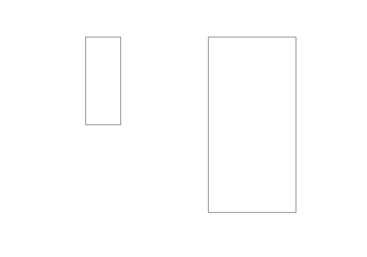
plot(TwoPolys)

plot of chunk unnamed-chunk-6

Writing a shapefile

We can save our SpatialPolygons object as a shapefile using the raster package. The shapefile function in the raster package is very convenient in that it can both read a shapefile into R but it can also write a SpatialPolygons or other spatial object classes (lines, polygons, etc.) to a shapefile.

library(raster)
shapefile(x = TwoPolys, file = "path/to/output/file.shp")

Reading a SpatialPolygon from file

Creating 100s of polygons by hand is a very daunting task. Most people deal with SpatialPolygon files that have already been created and are read into R via a shapefile. In the next portion of this tutorial we’ll download a SpatialPolygonDataFrame that contains US State boundaries.

We can get the data directly from within R using the getData function available in the raster package.

# This looks up the GADM dataset - for the country US and returns 
# the first level of administration which in this case is state boundaries. 

States <- raster::getData("GADM", country = "United States", level = 1)

# Have a look at the data
States

## class       : SpatialPolygonsDataFrame 
## features    : 51 
## extent      : -179.1506, 179.7734, 18.90986, 72.6875  (xmin, xmax, ymin, ymax)
## crs         : +proj=longlat +datum=WGS84 +no_defs +ellps=WGS84 +towgs84=0,0,0 
## variables   : 10
## names       : GID_0,        NAME_0,   GID_1,  NAME_1, VARNAME_1, NL_NAME_1,           TYPE_1,        ENGTYPE_1, CC_1, HASC_1 
## min values  :   USA, United States, USA.1_1, Alabama, AK|Alaska,        NA, Federal District, Federal District,   NA,  US.AK 
## max values  :   USA, United States, USA.9_1, Wyoming,   WY|Wyo.,        NA,            State,            State,   NA,  US.WY

We can see that the States object is a SpatialPolygonsDataFrame. It contains spatial information about the state boundaries but also additional data like the name and some other things.

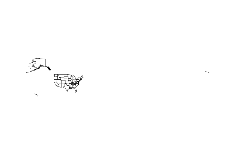
Plot this to see that it looks like

plot(States)

plot of chunk unnamed-chunk-7

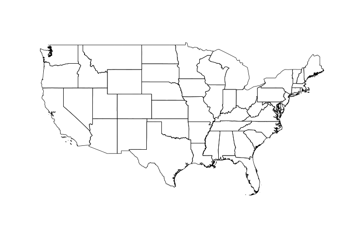
For plotting purposes let’s subset out Alaska and Hawaii from the current data

States <- States[States$NAME_1 != "Alaska" & States$NAME_1 != "Hawaii",]

plot of chunk unnamed-chunk-9

Dissolving boundaries

Often we find that we have lots of spatial polygons that represent the same information. For example, let’s say you have a very fine scale polygon shapefile of the United States. Each island or disjunct polygon will become it’s own polygon within the larger data set. Let’s imagine that you want to extract values for a particular state - Alaska for example. Each individual Aleutian island will be it’s own polygon and thus when summarizing data each island will have it’s own mean. We can get around that by dissolving boundaries based on similar attributes. Essentially collapsing multiple polygons into a single polygon.

Here we’re going to dissolve the state boundaries to make a single United States (lower 48) border polygon. We’ll use the rgeos package to do that. Make sure you have it installed.

library(rgeos)

## rgeos version: 0.5-1, (SVN revision 614)
##  GEOS runtime version: 3.5.0-CAPI-1.9.0 
##  Linking to sp version: 1.3-1 
##  Polygon checking: TRUE

Within the rgeos package there are lots of handy spatial functions. We’ll use a special case of the gUnion function to dissolve our state boundaries. In order to dissolve we need a common identifier in all the polygons we want to ‘merge’ together. The ISO field is the same for all polygons. We’ll use that to dissolve boundaries into one polygon.

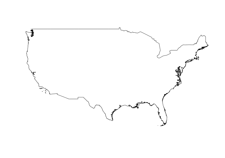
USborder <- rgeos::gUnaryUnion(States, id = States$ISO)

Take a look at the new single polygon

# What does it look like
USborder

## class       : SpatialPolygons 
## features    : 1 
## extent      : -124.7628, -66.94889, 24.52042, 49.3833  (xmin, xmax, ymin, ymax)
## crs         : +proj=longlat +datum=WGS84 +no_defs +ellps=WGS84 +towgs84=0,0,0

# Plot it
plot(USborder)

plot of chunk unnamed-chunk-12

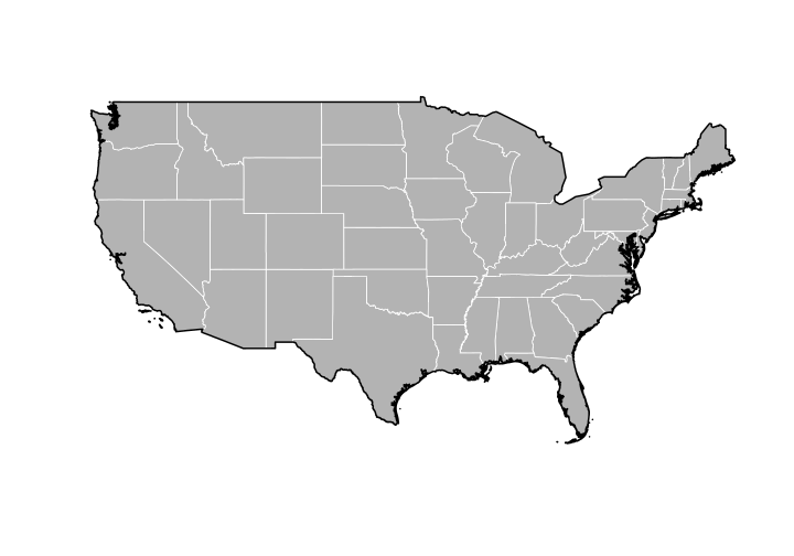
Let’s make a map using the newly created USborder and the state level data.

plot(States, 
     col = "gray70", # fill color
     border = "white") # outline color
plot(USborder, 
     lwd = 2,
     add = TRUE) # add to current plot

plot of chunk unnamed-chunk-13
Back to top