Introduction to spatial data analysis using the tidyverse

Authors: Clark S. Rushing
Contributors: Michael T. Hallworth

Installing Required Libraries

The libraries needed for these activities are: sf tidyverse maps

Installing the packages

If installing these packages for the first time consider adding dependencies=TRUE

install.packages("sf",dependencies = TRUE)

install.packages("tidyverse",dependencies = TRUE)

install.packages("maps",dependencies = TRUE)

This activity will integrate spatial data with the tidyverse. See introduction to the tidyverse for more information on the tidyverse.

Download R script Last modified: 2019-09-20 18:26:28

The tidyverse and spatial data

Compared to other data science topics, analysis of spatial data using the tidyverse is relatively underdeveloped. Because the common spatial packages (sp, rgdal, and rgeos) use S4 objects to represent spatial data, they do not play nice with the tidyverse packages (which require data frames). However, the powerful new spatial package sf is starting to bridge the divide. sf stands for ‘Simple Features’, which is the open source standard for spatial data used by many GIS software programs. Unlike the other spatial packages, sf is built around data frames, so manipulation of sf objects is generally more intuitive (relative to S4 objects) even if you don’t want to use the tidyverse. However, as we’ll see throughout this tutorial, integrating spatial analysis with tidyverse workflows has many advantages.

Several good resources are available for learning more about Simple Features objects and the sf packages, including the package vignette, the forthcoming book Geocomputation in R by Lovelace, Nowosad, & Muenchow, and this great blog post by Jesse Sadler. This activity borrows heavily from these three sources. They are excellent references.

Because sf appears to be the future of spatial analysis in R, especially with regards to the tidyverse, we will start with a brief introduction to the structure, creation, and (quick) visualization of sf objects in R.

Structure of sf objects

The sf package implements the Simple Features standard in R. The Simple Features standard is used to represent geographic vector data (sorry, no raster support right now) by many GIS software, including PostGIS, GeoJSON, and ArcGIS. A simple feature contains, at a minimum, a geometry that includes the coordinates of one or more points. Simple features may also contain (and often do) lines connecting the points, a CRS, and attributes associated with each geographic element. To illustrate the structure of sf objects, we will start by manually creating a very simple point object containing coordinates and attributes of several cities in Arizona.

The basic units of sf objects are called sfg objects. sfg objects provide the coordinates, dimension, and type of geometry for a single spatial feature. The sf package supports seven geometry types (which should be pretty self-explanatory):
- POINT
- MULTIPOINT
- LINESTRING
- MULTILINESTRING
- POLYGON
- MULTIPOLYGON
- GEOMETRYCOLLECTION (any combination of the other 6 types)

To manually create any of the seven geometries, we use the corresponding functions st_point(), st_linestring(), st_multipoint(), etc. (Note that all functions in the sf package start with st_). We will use the st_point() function to create individual sfg objects for four Alaskan cities. At a minimum, sf_point() requires a vector containing the longitude and latitude (in that order!) of each point:

library(sf)
library(tidyverse)

ju_sfg <- st_point(c(-134.4333, 58.3059)) #Juneau
an_sfg <- st_point(c(-149.8631, 61.2174)) #Anchorage
fa_sfg <- st_point(c(-147.7767, 64.8354)) #Fairbanks
nm_sfg <- st_point(c(-165.4064, 64.5011)) #Nome

On your own:

Print one of the sfg objects. What do you see? Hopefully, you see that it is POINT geometry and the coordinates of the point in parentheses.

To extract the coordinates of an sfg object, use the sf_coordinates() function:

st_coordinates(ju_sfg)

##           X       Y
## 1 -134.4333 58.3059

To create MULTIPOINT or LINESTRING sfg objects, we combine the coordinates of the individual points into a matrix, which is then used as the input argument to the corresponding functions:

## Create MULTIPOINT object
ak_sfg <- st_multipoint(rbind(c(-134.4333, 58.3059), 
                              c(-149.8631, 61.2174),
                              c(-147.7767, 64.8354),
                              c(-165.4064, 64.5011)))

# Create LINESTRING object
ak_sfg <- st_linestring(rbind(c(-134.4333, 58.3059), 
                              c(-149.8631, 61.2174),
                              c(-147.7767, 64.8354),
                              c(-165.4064, 64.5011)))

On your own:

Print these new objects and compare the structure to the structure of the POINT objects.

Back to top

sfc class objects

The sfg objects we created contain coordinates and the geometry type of spatial objects but sfg objects are not truly geospatial objects because they lack a coordinate reference system (CRS). The sf package uses another object class called sfc to add a CRS to one or more sfg objects (you have already learned about coordinate reference systems in R so we will not review that here). To create a sfc object, we use (you guessed it) the st_sfc function:

st_sfc takes one or more sfg objects (in this case, POINT objects for each of our cities), and (optionally) a crs attribute, which can be an epsg code or a proj4string string (remember those?). In this case, we use epsg 4236, which corresponds to latitude and longitude coordinates on the WGS84 ellipsoid. The crs, epsg, geometry type, dimensions, and individual sfg objects can be viewed by printing the sfc object in the console.

cities_sfc <- st_sfc(ju_sfg, an_sfg, fa_sfg, nm_sfg, crs = 4326)
cities_sfc

## Geometry set for 4 features 
## geometry type:  POINT
## dimension:      XY
## bbox:           xmin: -165.4064 ymin: 58.3059 xmax: -134.4333 ymax: 64.8354
## epsg (SRID):    4326
## proj4string:    +proj=longlat +datum=WGS84 +no_defs

Challenge:

What happens in you do not provide a CRS as an argument to st_sfc?

To access the CRS of an sfc object, use the st_crs() function:

st_crs(cities_sfc)

## Coordinate Reference System:
##   EPSG: 4326 
##   proj4string: "+proj=longlat +datum=WGS84 +no_defs"

sfc objects can also be easily visualized (in this case the plot is admittedly not very interesting, but this is just to show that you can do it):

plot(cities_sfc)

sf objects

The sfc object we created above contains all of the geospatial data associated with our points but generally we want to also include attributes along with the spatial data. This is where full-blown sf objects come in handy. As described above, one of the advantages of sf objects is that they are just data frames, more or less the same as every other data frame you’ve worked with in R. Lets add a few attributes to our city sfc object:

# Create data.frame with attributes
cities_df <- data.frame(Name = c("Juneau", "Anchorage", "Fairbanks", "Nome"),
                        Population = c(31276, 291826, 3598, 31535),
                        Elevation = c(17, 31, 6, 136))

# Combine data.frame and spatial data
cities_sf <- st_sf(cities_df, geometry = cities_sfc)

sf_sf can take a variety of input. In this case, we provided a data.frame object and an sfc object of the same length. We also named the sfc column ‘geometry’, which will allow our new object to play nice with some of the tidyverse functions later. If you don’t explicitly name the sfc column, it will be named after the sfc object. Let’s look at the structure of our new object:

cities_sf

## Simple feature collection with 4 features and 3 fields
## geometry type:  POINT
## dimension:      XY
## bbox:           xmin: -165.4064 ymin: 58.3059 xmax: -134.4333 ymax: 64.8354
## epsg (SRID):    4326
## proj4string:    +proj=longlat +datum=WGS84 +no_defs
##        Name Population Elevation                  geometry
## 1    Juneau      31276        17 POINT (-134.4333 58.3059)
## 2 Anchorage     291826        31 POINT (-149.8631 61.2174)
## 3 Fairbanks       3598         6 POINT (-147.7767 64.8354)
## 4      Nome      31535       136 POINT (-165.4064 64.5011)

Like the sfc objects, printing an sf object displays the spatial information (geometry type, dimension, crs). Beneath this information, it also prints the newly created data frame containing the attribute and geometry data. This object is almost just like any other data frame you have used in R but it does have a few important differences. We can see the first by looking at the class of the sf object:

class(cities_sf)

## [1] "sf"         "data.frame"

So cities_sf has both sf and data.frame classes. The sf class contains the geospatial data that we saw by printing the object. The data.frame contains all of the data. It is also informative to look at the structure of cities_sf:

str(cities_sf)

## Classes 'sf' and 'data.frame':	4 obs. of  4 variables:
##  $ Name      : Factor w/ 4 levels "Anchorage","Fairbanks",..: 3 1 2 4
##  $ Population: num  31276 291826 3598 31535
##  $ Elevation : num  17 31 6 136
##  $ geometry  :sfc_POINT of length 4; first list element:  'XY' num  -134.4 58.3
##  - attr(*, "sf_column")= chr "geometry"
##  - attr(*, "agr")= Factor w/ 3 levels "constant","aggregate",..: NA NA NA
##   ..- attr(*, "names")= chr  "Name" "Population" "Elevation"

The first three columns are what you would expect: one factor (Name) and two numeric (Population & Elevation) vectors. But geometry is different. It is actually a ‘list-column’, meaning that each element (i.e., row) of the column contains a list. It is identical to the cities_sfc object, with each element containing the sfg object associated with each city (see how that all came together?).

Back to top

Creating sf objects from other Spatial objects

Although it’s useful to create an sf object from scratch, this process would be too cumbersome for real-world spatial objects. Luckily, st_as_sf() can be used to convert other types of spatial objects to class sf. For example, ket’s create a polygon containing the borders of Alaska from a shapefile:

ak <- raster::shapefile("../Spatial_Layers/ak.shp")
class(ak)

## [1] "SpatialPolygonsDataFrame"
## attr(,"package")
## [1] "sp"

We can see that ak is a SpatialPolygonsDataframe. Next, let’s convert ak to a sf object and set the CRS:

### Covert from SpatialPolygonsDataframe to sf
ak_sf <- st_as_sf(ak)


### Set CRS to WGS84
ak_sf <- st_transform(ak_sf, crs = 4326)

### View object
ak_sf

## Simple feature collection with 1 feature and 1 field
## geometry type:  MULTIPOLYGON
## dimension:      XY
## bbox:           xmin: -179.1335 ymin: 51.24227 xmax: -129.9795 ymax: 71.35043
## epsg (SRID):    4326
## proj4string:    +proj=longlat +datum=WGS84 +no_defs
##   FID                       geometry
## 0   0 MULTIPOLYGON (((-179.0905 5...

Note that to view the CRS of a sf object, use the st_crs() function. But to set the CRS of an existing object, use st_transform().

Once we have an sf object, manipulation using the tidyverse is straightforward. Now let’s make a map.

Back to top

Basic maps using ggplot2

As you have already seen, R has many tools for making nice maps that do not use the tidyverse. But the tidyverse contains a powerful visualization package: ggplot2. ggplot2 is built on the ‘grammar of graphics’ - basically a set of rules for building visualizations piece by piece. Although daunting at first, ggplot2 provides unparalleled flexibility for making publication-quality graphics, including maps.

To use ggplot2 with sf objects, you will need the latest version of ggplot2. If you have not done so recently, be sure to update to the latest version:

install.packages("ggplot2")

The most recent version of ggplot2 gives us access to a new functionality: geom_sf(). Unlike other ggplot2 figures, where the user needs to specify a specific geometry (e.g., geom_point(), geom_polygon(), geom_path()), geom_sf() can plot different geometries depending on the geometry type of the sf object. geom_sf() requires a column called geometry (which is why we explicitly named the sfc object ‘geometry’ when we created our city sf object) and then it takes care of the rest:

library(ggplot2)
ggplot() +
  geom_sf(data = ak_sf) +     # Alaska border polygon
  geom_sf(data = cities_sf, color = "red", size = 3)   # Cities

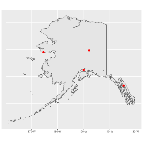
Not bad. Both the border polygon and cities are displayed nicely, the axis labels are automatically given the appropriate units, and the grid lines are displayed as graticules! That gray background isn’t too pretty but we can easily fix that by changing from the default theme to theme_minimal():

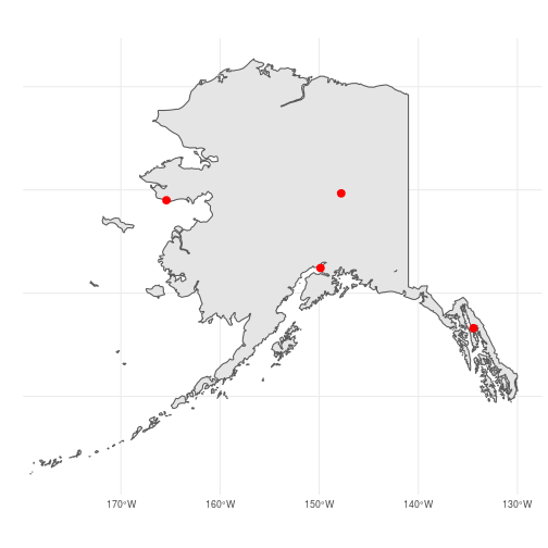
ggplot() +
  geom_sf(data = ak_sf) +
  geom_sf(data = cities_sf, color = "red", size = 3) + 
  theme_minimal()

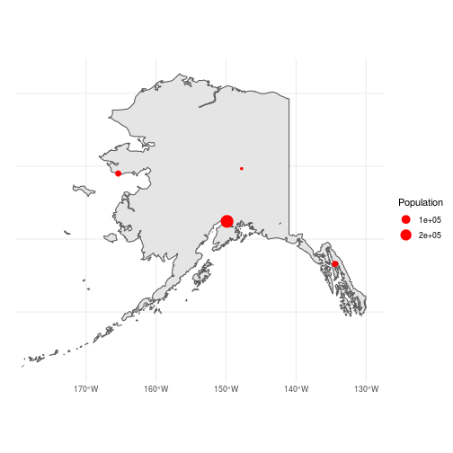
Next, let’s use some of the attributes to make our map more informative. With ggplot2 we can map attributes to the aesthetics (size, shape, color, etc.) of the points using the aes() argument inside geom_sf(). We’ll make use point size to show differences in population size of the cities by setting size = Population:

ggplot() +
  geom_sf(data = ak_sf) +
  geom_sf(data = cities_sf, color = "red",
          aes(size = Population), 
          show.legend = "point") + 
  theme_minimal()

Finally, let’s label the cities. In ggplot2, this can be done using geom_text() and mapping the Name column in cities_sf to the text labels (i.e., aes(label = Name)). One issue, though, is that geom_text() needs columns containing the x & y coordinates of each point. In our sf object, those coordinates are buried deep down in the geometry column so we need to extract them and create new x/y columns for geom_text(). In the tidyverse, adding columns is done using the dplyr function mutate() (for more information about the arguments, see the help file using ?mutate). Perhaps the easiest way to add x and y columns would be to manually create vectors containing the longitude and latidude of each city and supply those vectors as arguments to mutate(). That method, however, doesn’t generalize very well to situations where you didn’t create the sf object from scratch. A better option is to directly extract the coordinates using the map_dbl() function from the tidyverse package purrr (note that rather than loading purrr for a single function, we use the :: option tell R that map_dbl is from the purrr package). Remember, each element of the geometry column is a list. map_dbl takes a list as the first argument, applies a function to each element, and returns a vector containing the output from function. In the code below, we give a numeric value instead of a function, which tells map_dbl to extract the corresponding element within each list. In this case, we are telling mutate() to create two new columns called x and y. For each column, we tell map_dbl to extract either the 1st (longitude) or 2nd (latitude) coordinate for each point:

cities_sf <- mutate(cities_sf, 
                    x = purrr::map_dbl(geometry, 1), 
                    y = purrr::map_dbl(geometry, 2))

ggplot() +
  geom_sf(data = ak_sf) +
  geom_sf(data = cities_sf, color = "red",
          aes(size = Population), 
          show.legend = "point") + 
  geom_text(data = cities_sf, 
            aes(x = x, y = y, 
                label = Name), hjust = 1.2) +
  theme_minimal() +
  theme(axis.title = element_blank())

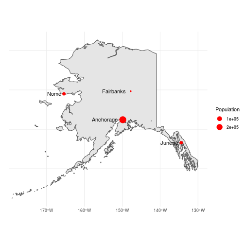
There may be many other tweaks we would make before being satisfied with this map but this is not a bad start for just a few lines of code.

Back to top