
Spatial Predicates
Contributors: Clark S. Rushing
R Skill Level: Intermediate - this activity assumes you have a working knowledge of R
Objectives & Goals
Upon completion of this activity, you will:- know to clip features
- know how to find where features intersect
- know how to dissolve features
- be able to determine if features are within / contain other features
- be able to calculate the area of a feature
Required packages
To complete the following activity you will need the following packages installed: raster sp rgeosInstalling the packages
If installing these packages for the first time consider addingdependencies=TRUE
install.packages("raster",dependencies = TRUE)install.packages("rgdal",dependencies = TRUE)install.packages("rgeos",dependencies = TRUE)install.packages("sp",dependencies = TRUE)Download R script Last modified: 2019-09-20 18:26:28
Spatial predicates
Spatial predicates are a series of spatial relations between two or more spatial features. The table below gives simple definitions for the predicate and the accompanying function in the rgeos package. The sf package also has similar functions.
| Predicate | Definition | Function |
|---|---|---|
| Equals | Geometries are equivilant | gEquals() |
| Disjoint | No commonality in geometries | gIntersects() |
| Touches | Geometries have one common boundary point | gTouches() |
| Contains | Geometry is contained by or contains another geometry | gContains() |
| Covers | Geometry a is covered by b |
gCovers() |
These functions can be very helpful and are commonly performed functions in GIS.
Before we get started we’ll load the libraries that we need for this activity.
library(raster)
library(sp)
library(rgeos)
Clipping a polygon
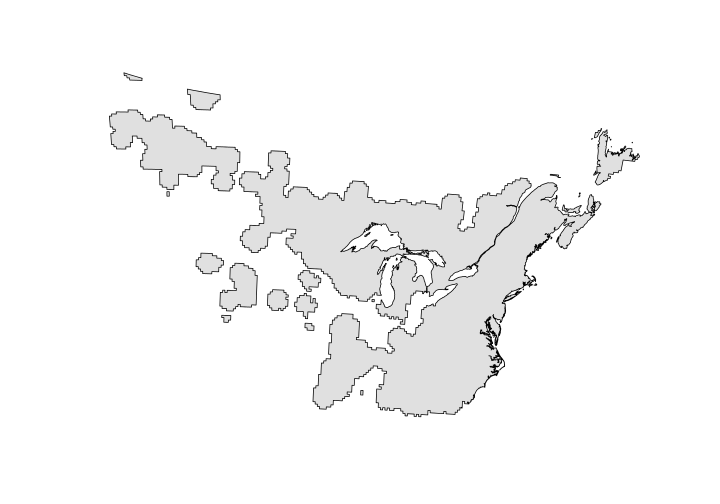
Clipping one polygon by another is a fairly common GIS procedure that you may have done in the past. To demonstrate how we can do this in R we’ll use a species distribution map to clip the United States to determine which states the species distribution includes. We’ll learn some new techniques along the way. For instance we’ll encounter the function used to dissolve boundaries. We’ll clip a polygon and then find the area of the overlapping polygons.
First, we need to get a polygon file of the United States.
# Download or read in states polygon
States <- getData("GADM",country = "United States", level = 1)
Next, let’s grab a polygon shapefile of the Ovenbird distribution from the Breeding Bird Survey’s website.
# Use the download.file function -
# Don't forget the destfile = "path/where/to/store/file"
download.file(url = "https://www.mbr-pwrc.usgs.gov/bbs/ra15/ra06740.zip",
              destfile = "../Spatial_Layers/ovenbird.zip")
The file should have downloaded. Let’s check to see that the file downloaded properly.
file.exists("../Spatial_Layers/ovenbird.zip")
## [1] TRUE
Now let’s unzip the file and see what’s in it.
# unzip the zipped folder
# exdir - where do you want to put the
#         unzipped files

unzip(zipfile = "../Spatial_Layers/ovenbird.zip",
      exdir = "../Spatial_Layers/ovenbird")

# take a look at the files
list.files("../Spatial_Layers/ovenbird")
## [1] "ra06740.dbf" "ra06740.prj" "ra06740.shp" "ra06740.shx"
Let’s read in the Ovenbird’s distribution
OVEN <- raster::shapefile("../Spatial_Layers/ovenbird/ra06740.shp")

# have a look
OVEN
## class       : SpatialPolygonsDataFrame
## features    : 10890
## extent      : -1900596, 3106908, 1075820, 4325680  (xmin, xmax, ymin, ymax)
## crs         : +proj=aea +lat_1=29.5 +lat_2=45.5 +lat_0=23 +lon_0=-96 +x_0=0 +y_0=0 +datum=NAD83 +units=m +no_defs +ellps=GRS80 +towgs84=0,0,0
## variables   : 6
## names       :       AREA, PERIMETER, TMPCOV_, TMPCOV_ID, GRID_CODE,   RASTAT
## min values  :   433703.6,  3037.274,      10,         0,         0,        0
## max values  : 1389074000,  172282.4,    9999,      9999,     38112, 70.57192
Dissolving features
One thing you should notice is that there are a ton of polygons. There are 10890 different polygons! Let’s dissolve the boundaries so we have only a single polygon. In order to do that we need to make sure we have a variable within OVEN that is shared by all features. Looks like we’ll need to create one.
# make a variable used to dissolve boundaries
OVEN$dissolve <- 1
Now that we have that field we can use the gUnaryUnion function to make a single polygon.
#Dissolve boundaries
OVEN_single_poly <- rgeos::gUnaryUnion(OVEN,
                                       id = OVEN$dissolve)

# take a look
OVEN_single_poly
## class       : SpatialPolygons
## features    : 1
## extent      : -1900596, 3106908, 1075820, 4325680  (xmin, xmax, ymin, ymax)
## crs         : +proj=aea +lat_1=29.5 +lat_2=45.5 +lat_0=23 +lon_0=-96 +x_0=0 +y_0=0 +datum=NAD83 +units=m +no_defs +ellps=GRS80 +towgs84=0,0,0
Here we’ll use the gIntersection function in the rgeos package. The rgeos package can recognize that the coordinate reference systems differ between our two polygon files. It should give you a warning and proceed. Make sure to include byid = TRUE otherwise you only get a single polygon return - and it takes 15 times longer!
The intersect function in the raster package is a little slower than the gIntersection function in the rgeos package. The one huge advantage to using raster’s intersect is that it preserves associated data in a SpatialPolygonsDataFrame.
# Project states into same CRS
States_aea <- sp::spTransform(States,sp::CRS(OVEN_single_poly@proj4string@projargs))

# Find the intersection using rgeos
a<-Sys.time()
OVENstates_rgeos <- rgeos::gIntersection(spgeom1 = OVEN_single_poly,
                                         spgeom2 = States_aea,
                                         byid = TRUE,
                                         id = States_aea$NAME_1)
Sys.time()-a
## Time difference of 5.967775 secs
# Find the intersection using raster
a<-Sys.time()
OVENstates_raster <- raster::intersect(x = OVEN_single_poly,
                                       y = States_aea)
Sys.time()-a
## Time difference of 7.459309 secs
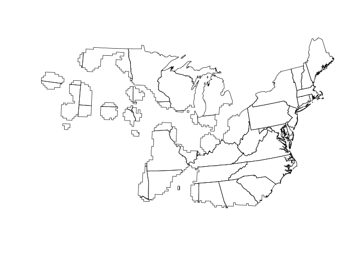
Now that we have a clipped polygon, let’s determine the area of each state that the Ovenbird distribution overlaps. To do this we’ll use the gArea function in the rgeos package. First, let’s see how much area the Ovenbird’s distribution encompasses.
OVEN_area <- rgeos::gArea(OVEN_single_poly)/10000
Find area of each state. Here we set byid = TRUE to get the area of each state.
# Here we set byid = TRUE
State_area <- rgeos::gArea(OVENstates_raster, byid = TRUE)/10000
Combining the output into a data frame.
# Get states within their distribution
State_area <- data.frame(State = OVENstates_raster$NAME_1,
                         Area_km = State_area)

head(State_area)
##                  State    Area_km
## 1              Alabama 6465488.15
## 2          Connecticut 7821423.16
## 3 District of Columbia  415567.39
## 4              Georgia 1285287.29
## 5             Illinois  515468.08
## 6              Indiana   16607.04