Extracting raster data
Contributors: Clark S. Rushing
R Skill Level: Intermediate - this activity assumes you have a working knowledge of R
This activity incorporates the skills learned in the Points, Polygons, Raster & Projections activities.
Objectives & Goals
Upon completion of this activity, you will:- know how to generate isoptope assignments
- know how to perform basic raster calculations
Required packages
To complete the following activity you will need the following packages installed: raster sp rgeosInstalling the packages
If installing these packages for the first time consider addingdependencies=TRUE
install.packages("raster")
install.packages("velox")
install.packages("sp")
install.packages("rgeos")
Download R script Last modified: NA
library(raster)
library(velox)
library(sp)
library(rgeos)
Gathering spatial data
First we need a raster with the predicted stable-isotope of Hydrogen in precipitation. We can get that from waterisotopes.org. Below we use R to download the file and unzip it for us.
# Download the file #
utils::download.file(url = "http://wateriso.utah.edu/waterisotopes/media/ArcGrids/AnnualD.zip",
                     destfile = "../Spatial_Layers/AnnualD.zip",
                     quiet = TRUE,
                     extra = getOption("download.file.extra"))

# unzip the downloaded file #
utils::unzip(zipfile = "../Spatial_Layers/AnnualD.zip",
            files = NULL, list = FALSE, overwrite = TRUE,
            junkpaths = FALSE, exdir = "../Spatial_Layers", unzip = "internal",
            setTimes = FALSE)

# remove the zipped file to by tidy
file.remove("../Spatial_Layers/AnnualD.zip")
## [1] TRUE
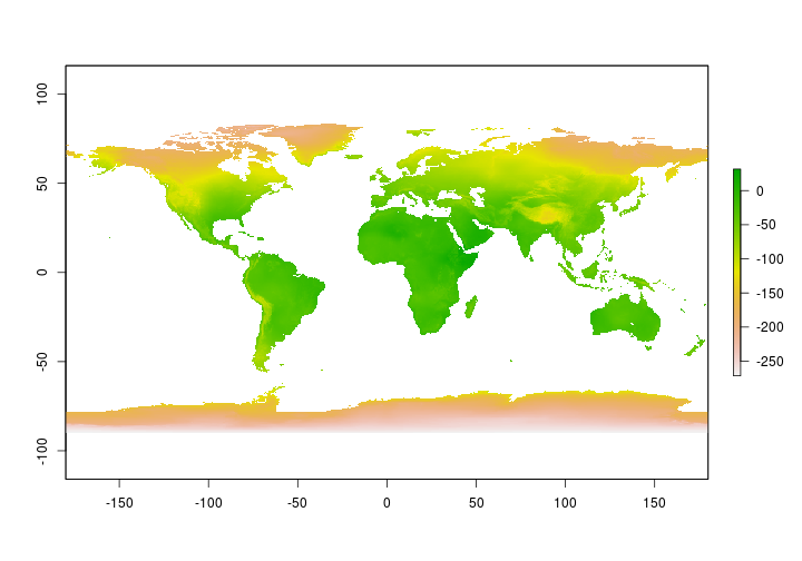
Read in the predicted surface for Hydrogen isotopes in precipitation. Generally, in North America Hydrogen isotope values are more depleted (more negative) in the north and more enriched (less negative). The plot below shows that pattern.
# read in Mean Annual D #
m_a_d <- raster::raster("../Spatial_Layers/AnnualD/mad/w001001.adf")
Now that we have the base layer we need to determine the discrimination factor between the isotope values precipitation and the measured isotope values in the tissue of interest. Here, we’ll simulate some data using techniques we learned in other lessons.
Simulate ‘known’ values from capture location
To simulate these data we’ll first need capture locations that fall within the region of interest. For this exercise we’ll simulate 10 captures at 10 sites within the United States. Once we have the capture locations, we will extract the isotope value in precipitation. We’ll then simulate ‘measured’ isotope values - we’ll add a little noise to be more realistic.
# Read in a shapefile of the United States #
States <- raster::getData("GADM", country = "United States", level = 1)

# remove Alaska and Hawaii for this simulation (sorry) #

States <- States[!(States$NAME_1 %in% c("Alaska","Hawaii")),]

# dissolve all states so only have the border
USborder <- rgeos::gUnaryUnion(States, id = States$ISO)
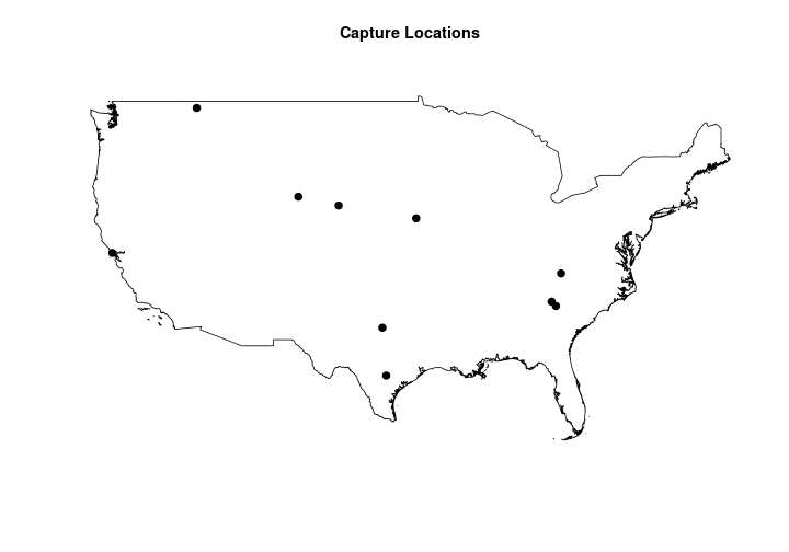
Now that we have a boundary for the contiguous United States we can generate 10 randomly generated capture locations.
# Set the random seed generator
set.seed(12345)

# Generate capture locations for calibration
CalibCapLocs <- sp::spsample(x = USborder, n = 10, type = "random")
Extract precipitation values
Now that we have capture locations we’ll extract the predicted isotope values in precipitation.
# extract estimated H in precipitation
estHp <- raster::extract(m_a_d, CalibCapLocs)
Here are the predicted Hydrogen values in precipitation.
##  [1]  -32.96  -34.04 -117.70 -109.95  -51.22  -31.44  -75.62  -44.69
##  [9]  -24.39  -80.26
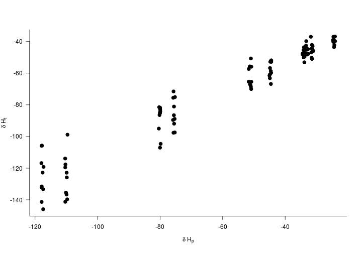
Simulate ‘measured’ tissue values
If the tissue values matched the precipitation values exactly making assignments would be pretty straightforward. Here we’ll add a little realism by adding some noise to the estimated value plus account for isotopic discrimination as they move through the food web. We’ll simulate 10 individuals at every capture location.
# set seed for random sampling
set.seed(12345)

# Make a data frame to store the data
Hvalues <- data.frame(Hp = rep(estHp,each =10), # H in precip
                      Ht = NA)                  # H in tissue

# known slope
knownBeta <- 0.93
Beta.sd <- 0.1

# known intercept
knownAlpha <- -15
Alpha.sd <- 0.2

# y = mx+b with some wiggle
Hvalues$Ht <- Hvalues$Hp*rnorm(knownBeta,n = 100, sd = Beta.sd)+rnorm(knownAlpha,n=100, sd = Alpha.sd)
Discrimination factor
Now that we’re finished simulating data we can begin the analysis. First we’ll use the simulated data to generate a discimination factor. In other words we need to determine how the tissue isotope signatures are related to the precipitation signatures. We’ll do this using a linear model so that we can make geographic assignments for individuals from unknown origins.
# discrimination factor
fit <- lm(Hvalues$Ht~Hvalues$Hp)
##
## Call:
## lm(formula = Hvalues$Ht ~ Hvalues$Hp)
##
## Residuals:
##      Min       1Q   Median       3Q      Max
## -21.0870  -3.9547  -0.9672   4.7238  21.8448
##
## Coefficients:
##              Estimate Std. Error t value Pr(>|t|)
## (Intercept) -14.57726    1.70911  -8.529 1.86e-13 ***
## Hvalues$Hp    0.96013    0.02505  38.329  < 2e-16 ***
## ---
## Signif. codes:  0 '***' 0.001 '**' 0.01 '*' 0.05 '.' 0.1 ' ' 1
##
## Residual standard error: 8.031 on 98 degrees of freedom
## Multiple R-squared:  0.9375,	Adjusted R-squared:  0.9368
## F-statistic:  1469 on 1 and 98 DF,  p-value: < 2.2e-16
below we extract the information we need to make isotope assignments. First, we’ll need the intercept and slope from the linear equation above.
# extract the slope from lm oject
slope <- fit$coefficients[2]

# extract intercept from lm object
int <- fit$coefficients[1]
create a tissue-isoscape
Now that we know the relationship between our tissue of interest (say a tail feather) and the precipitation isoscape we can create a ‘tissue-isoscape’ to make predictions.
# make the tissue-isocape using y = mx+b
Tissue_isoscape <- m_a_d*slope+int
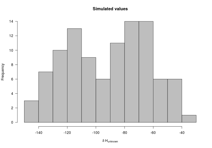
Great - now we’ll use this discrimination factor to make predictions for 100 individuals captured in the non-breeding season. First we need to simulate those values. In this simulation we’ll assume weak migratory connectivity where a single capture location in the non-breeding season is home to individuals from across the breeding distribution - similar to the Prothonotary warbler (see Tonra et al. 2019).
# simulate 100 tail feather values
unk_Ht <- runif(n = 100, min = min(Hvalues$Ht), max = max(Hvalues$Ht))
Making geographic assignments
Now that we 1) know the discrimination factor and 2) have a tissue-isoscape we are almost ready to make geographic assignments. First we need to understand what we are about to do. Below we make probabilistic geographic assignments based on a normal probability density function. The mean of the normal is the ‘measured’ tissue value. The location uncertainty is determined by the standard deviation. We derive the standard deviation using the standard deviation of the residuals from our discrimination function above.
Let’s extract the standard deviation of the residuals first.
(StdDev <- sd(fit$residuals))
## [1] 7.990335
Below is a figure of the general concept for how we make assignments.
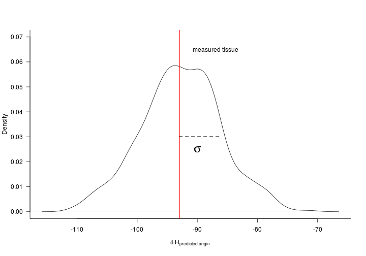
Now let’s apply the normal probability density function to a raster so that we can make spatially explicit assignments. The spatially explicit assignments are made where the likelihood that each ‘unknown’ tissue value, $y^*$, originates from a given location is
where $\mu_b$ is the specific cell in a given tissue isoscape and $\sigma_b$ is the standard deviation of the residuals from the discrimination equation.
Let’s make a function that we’ll call assign that makes the assignments for us.
# spatially explicit assignment function
assign <- function(isotope,isoscape,std) {
          ((1/(sqrt(2 * 3.14 * std))) * exp((-1/(2 * std^2)) * ((isotope) - isoscape)^2))
           }
Let’s make our first geographic assignments
# Let's get an approximate idea where the
# first individual molted

MoltEst <- assign(isotope = unk_Ht[1],
                   isoscape = Tissue_isoscape,
                   std = StdDev)
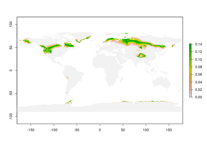
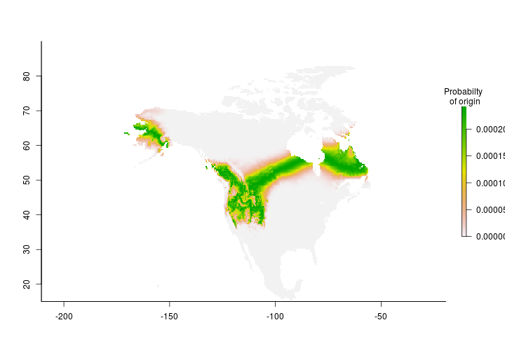
Great - now we have our first isotope assignment but we make predictions for the entire planet. Let’s confine our estimates to include only North America since our ‘study’ species isn’t found anywhere else during the breeding season.
Coming soon
Assignments using the MigConnectivity package