Spatial Interpolation

Authors: Michael T. Hallworth
Contributors: Clark S. Rushing

This activity will introduce you to spatial interpolation in R.

R Skill Level: Intermediate - this activity assumes you have a working knowledge of R

This activity incorporates the skills learned in the Points, Raster & Projections activities.

In case you missed it

SpatialPoints
Rasters
Projections

---

Objectives & Goals

Upon completion of this activity, you will:

• know how to interpolate using inverse distance weighting
• know how to use ordinary kriging to predict across a surface

Required packages

To complete the following activity you will need the following packages installed: raster sp gstat spatstat

Installing the packages

If installing these packages for the first time consider adding

dependencies=TRUE

install.packages("raster")

install.packages("sp")

install.packages("gstat")

install.packages("spatstat")

Download R script Last modified: 2019-09-20 18:26:28

---

This is still very much a work in progress

One basic principle of geography is that variables that are close in space typically have similar values. We can use this principle to make predictions and interpolate a smooth surface from data sampled at points. There are a few ways to do this. Generally, when people refer to ‘kriging’ they are referring to interpolation.

The following examples will use the raw number of species detected along breed bird survey (BBS) routes within Arizona. The data were summarized for brevity but the data represent the number of species detected along each route through time. We didn’t do any formal analysis that accounts for imperfect detection. We just wanted some real data to illustrate interpolation.

library(raster)
library(sp)
library(gstat)
library(spatstat)

load("../Spatial_Layers/spproute.rda")

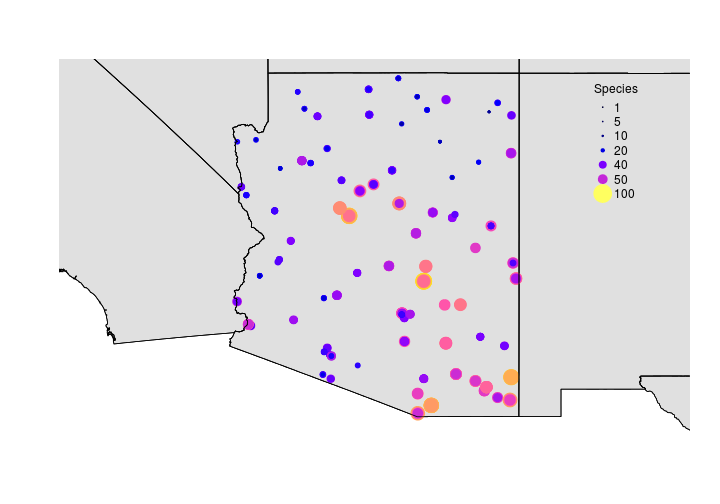
Now that we have some data let’s interpolate (predict values for locations were we have no data) species richness across Arizona.

Let’s make an empty raster so that we can predict species richness across AZ. We’ll use this several times so we’ll go ahead and make it here.

# Spatial grid over the extent of sppStateRoute
# approximately 5000 random points
# set.seed() makes sure the random points are the same each time
# increases reproducability 

set.seed(12345)
samplegrid <- raster::raster(sppStateRoute,res = c(0.025,0.025))

# define CRS
raster::crs(samplegrid) <- raster::crs(sppStateRoute) <- sp::CRS("+init=epsg:4326")

We’ll use the gstat package to interpolate species richness using a few different methods.

Inverse distance weighting

idw.model <- gstat(formula=sppStateRoute$SpeciesDetected~1, 
                   locations=sppStateRoute)

idw.spp <- raster::interpolate(samplegrid, idw.model)

## [inverse distance weighted interpolation]

## class      : RasterLayer 
## dimensions : 221, 222, 49062  (nrow, ncol, ncell)
## resolution : 0.025, 0.025  (x, y)
## extent     : -114.6683, -109.1183, 31.38823, 36.91323  (xmin, xmax, ymin, ymax)
## crs        : +init=epsg:4326 +proj=longlat +datum=WGS84 +no_defs +ellps=WGS84 +towgs84=0,0,0 
## source     : memory
## names      : var1.pred 
## values     : 11.42869, 75.10614  (min, max)

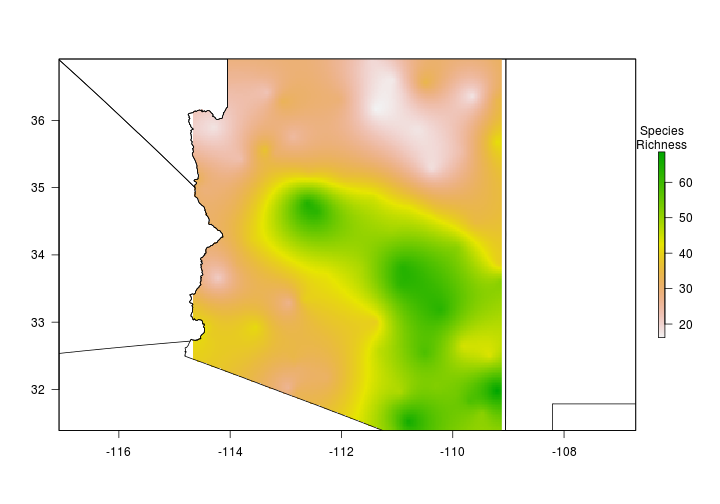
Let’s use the mask function to clip the raster to Arizona.

idw.spp.az <- raster::mask(idw.spp, States[States$NAME_1=="Arizona",])

par(bty="n",mar = c(0,0,0,0))
raster::plot(idw.spp.az,
             axes = FALSE,
             legend.args = list("Species\nRichness"))
plot(States, add = TRUE)

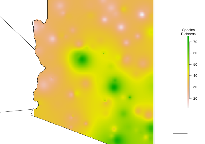
Ordinary Kriging

# remove duplicate locations because otherwise Kriging returns NA
sppStateRoute <- sppStateRoute[-sp::zerodist(sppStateRoute)[,1],]

# create variogram 
vario <- variogram(sppStateRoute$SpeciesDetected~1, sppStateRoute)

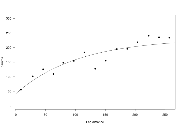
vario.fit <- fit.variogram(vario,
                           vgm(psill=250, # approx asymptote
                               range = 150,
                               model="Exp", 
                               nugget=50))

predict.model <- gstat(g=NULL,
                      formula = sppStateRoute$SpeciesDetected~1,
                      locations = sppStateRoute, 
                      model=vario.fit)

# make an empty raster to predict on #

r <- raster(ext = extent(sppStateRoute),
            res = c(0.025, 0.025), # same res as above
            crs = crs(sppStateRoute)@projargs)

# using ordinary kriging #
SpeciesRichness <- raster::interpolate(object = r, model = predict.model)

## [using ordinary kriging]

If you receive warnings that look similar to below, you have duplicate locations in your data. See above for how to remove duplicate locations.

Covariance matrix singular at location [-114.543,36.7882,0]: skipping...

back to top