Working with Point-Count like data
Contributors: Clark S. Rushing
R Skill Level: Intermediate - this activity assumes you have a working knowledge of R
Objectives & Goals
Upon completion of this activity, you will:- Generate random points within a polygon
- Create a buffer around the points
- Extract raster data to points
- predict occupancy and generate a surface using raster calculations
Required packages
To complete the following activity you will need the following packages installed: raster sp rgeosInstalling the packages
If installing these packages for the first time consider addingdependencies=TRUE
install.packages("raster",dependencies = TRUE)install.packages("rgdal",dependencies = TRUE)install.packages("rgeos",dependencies = TRUE)install.packages("sp",dependencies = TRUE)Download R script Last modified: 2019-09-20 18:26:28
Point-count like data
For this activity, let’s assume you’re getting ready to start a new project. In this project the primary form of data collection is through the use of point counts. Let’s assume you already know you want to survey birds within the Coronado National Forest the system in which you want to survey.
library(raster)
library(sp)
library(rgeos)
Read in a shapefile that contains information about the national forest boundaries in the United States. The shapefile was downloaded from here
# Read in Administrative forest boundaries
# This shapefile has boundary information
# for forests the U.S. federal govt is
# responsible for - i.e., National Forests,
# National Monuments, etc.

NatForest <- raster::shapefile("../Spatial_Layers/S_USA.AdministrativeForest.shp")

# Take a glance at the file
NatForest
## class       : SpatialPolygonsDataFrame
## features    : 112
## extent      : -150.0079, -65.69967, 18.03373, 61.51899  (xmin, xmax, ymin, ymax)
## crs         : +proj=longlat +datum=NAD83 +no_defs +ellps=GRS80 +towgs84=0,0,0
## variables   : 8
## names       :                           ADMINFORES, REGION, FORESTNUMB, FORESTORGC,                 FORESTNAME,     GIS_ACRES,      SHAPE_AREA,      SHAPE_LEN
## min values  :                       99010200010343,     01,         01,       0102,  Allegheny National Forest,     27566.061, 0.0120072002574, 0.754287568301
## max values  : e23b8205-a516-4aa3-945e-5dd93dbfe227,     10,         60,       1005, Willamette National Forest, 17684857.9312,   10.5984390953,  378.929375922
Let’s pull out just the Coronado National Forest. Here we use the grep() function to search for ‘Coronado’ within the FORESTNAME field.
CNF <- NatForest[grep(x=NatForest$FORESTNAME,pattern="Coronado"),]
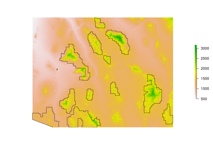
We’re going to need a Digital Elevation Model (DEM) for our analysis. For convience we’ll grab a DEM using the ‘alt’ (elevation) data set available with the raster package. Note - when using the raster to download elevation in the United States - a list is returned. The first element of the list is the elevation (in meters) of the contiguous states. The other elements include Alaska, and Hawaii.
# Get elevation data using the raster package
DEM <- raster::getData(name = "alt", country = "United States")
## returning a list of RasterLayer objects
# Save only the elevation in the lower 48
DEM <- DEM[[1]]
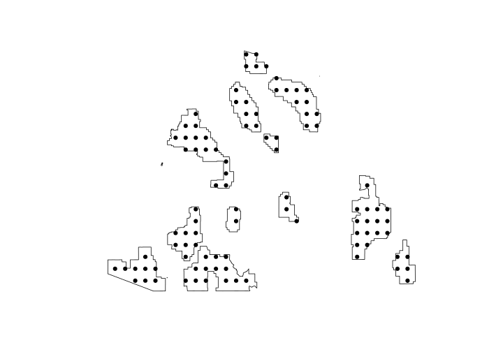
Generate point count locations
The sp package has a function to generate random points. It has a few options but here we’ll use type = "regular" to generate random points that are systematically aligned. The n is the approximate sample size. We’ll also set the seed for the random number generator so you should get the same locations.
set.seed(12345)

surveyPts <- sp::spsample(x = CNF, n = 100, type = "regular")
Let’s take a look at how many sites were generated and where they ended up.
plot(CNF)
plot(surveyPts, add = TRUE, pch = 19)
Generate buffer around points
Now that we have generate survey points - let’s make a 50m radius around each point.
Before we go any further we need to know a few things. We need to know if the coordinate reference system (crs) is defined for our survey points and we also need to what the crs is. To make our lives easier if would be good to have the surveyPoints projected into an Equal Area projection in meters. The reason for this is two-fold. First, an equal area projection will conserve area so our buffers should be accurate and second, if it’s in a meters we can specify the width parameter in meters.
surveyPts
## class       : SpatialPoints
## features    : 98
## extent      : -111.3911, -108.9843, 31.40503, 32.98191  (xmin, xmax, ymin, ymax)
## crs         : +proj=longlat +datum=NAD83 +no_defs +ellps=GRS80 +towgs84=0,0,0
Project the points into an equal area projection. While we’re at it - let’s project all our layers (DEM, forest boundaries, and survey points).
# Define the projection in proj4 format
EqArea <- "+proj=aea
           +lat_1=20 +lat_2=60 +lat_0=40 +lon_0=-96 +x_0=0 +y_0=0
           +ellps=GRS80
           +datum=NAD83
           +units=m +no_defs"

# project data using the sp package
surveyPts_m <- sp::spTransform(surveyPts, sp::CRS(EqArea))

# project forest boundary
CNF_m <- sp::spTransform(CNF, sp::CRS(EqArea))
Now for the DEM - it’s quite large and we only need a small portion. Let’s crop the DEM to include only the area around Coronado National Forest.
DEM <- crop(DEM,CNF)

# take a look
DEM
## class      : RasterLayer
## dimensions : 201, 304, 61104  (nrow, ncol, ncell)
## resolution : 0.008333333, 0.008333333  (x, y)
## extent     : -111.45, -108.9167, 31.33333, 33.00833  (xmin, xmax, ymin, ymax)
## crs        : +proj=longlat +ellps=WGS84
## source     : memory
## names      : USA1_msk_alt
## values     : 447, 3172  (min, max)
DEM_m <- projectRaster(DEM, crs = EqArea)
Now that we’ve projected the data we can generate the 50m radius around each point. To do this make sure to use byid = TRUE.
library(rgeos)
surveyCircle <- gBuffer(surveyPts_m, width = 50, byid = TRUE)
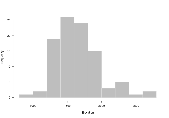
Extract elevation to the survey locations
pt_elev <- extract(DEM_m, surveyCircle, fun = mean, na.rm = TRUE)
Simulate count data
We’ll simulate occupancy data using a function from Kery & Royle 2016 Applied Hierarchical Modeling in Ecology. Here we use the simOcc function saving most of the preset values. We just want the count data so I save only the y ouput.
#library(AHMbook)
#library(unmarked)

# Simulate occupancy data
# M = number of sites
# J = number of occassions

simCount <- AHMbook::simOcc(M = length(surveyPts),
                            J = 3,
                            mean.occupancy = 0.6,
                            mean.detection = 0.7,
                            show.plot = FALSE)$y

# see first few rows
head(simCount)
##      [,1] [,2] [,3]
## [1,]    1    1    1
## [2,]    0    0    0
## [3,]    1    0    0
## [4,]    0    1    1
## [5,]    1    1    1
## [6,]    1    1    1
Using these simulated data, we’ll determine the relationship between elevation and occupancy while accounting for imperfect detection using the unmarked package.
# Make unmarked frame for occupancy data
umf <- unmarked::unmarkedFrameOccu(y = simCount,
                                   siteCovs=data.frame(pt_elev),
                                   obsCovs=NULL)

# run the occupancy model
occ <- unmarked::occu(~1~pt_elev,umf)
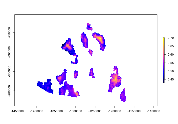
Map occupancy probability
Let’s create a map of the predicted occupancy probabilty throughout the Coronado National Forest. We’ll use the parameter estimates from the occupancy model we ran above.
occMap <- exp(unmarked::coef(occ)[1]+unmarked::coef(occ)[2]*DEM_m)/
          (1+exp(unmarked::coef(occ)[1]+unmarked::coef(occ)[2]*DEM_m))

plot(mask(occMap, CNF_m),col = bpy.colors(30))